Introduction and Theory

One of the biggest challenges of dynamical systems theory or nonlinear dynamics is the development of mathematical techniques that provide us with the capability of exploring the geometrical template of structures that governs transport in phase space. Since the early 1900, the idea of pursuing a qualitative description of the solutions of differential equations, which emerged from the pioneering work carried out by Henri Poincaré on the three body problem of celestial mechanics [1], has had a profound impact on our understanding of the nonlinear character of natural phenomena. Indeed, this powerful approach has now been widely embraced by the scientific community and its essence was nicely captured by Vladimir Arnold's statement that a complete description of classical mechanics boils down to the geometrical analysis of phase space.

In this section we present the details of a mathematical tool whose potential brings us one step closer to fulfilling the long sought after dream envisioned by Poincaré. The method is known in the literature as Lagrangian descriptors (LDs) and has the capability of revealing the geometrical template of phase space structures that characterizes trajectories with qualitatively distinct dynamical behavior. As we will see, this method provides us with a systematic way of exploring phase space by means of looking at its dynamical skeleton using low-dimensional slices. This procedure allows for a complete reconstruction, that is, a phase space tomography, of the intricate geometry of underlying invariant manifolds that characterize transport mechanisms.

Consider a general dynamical system:

\begin{equation} \dfrac{d\mathbf{x}}{dt} = \mathbf{v}(\mathbf{x},t) \;,\quad \mathbf{x} \in \mathbb{R}^{n} \;,\; t \in \mathbb{R} \;, \label{eq:gtp_dynSys} \end{equation}

where the vector field satifies $\mathbf{v}(\mathbf{x},t) \in C^{r} (r \geq 1)$ in $\mathbf{x}$ and continuous in time. If the vector field does not depend on time, the system is called autonomous, and it is non-autonomous otherwise. For any initial condition $\mathbf{x}(t_0) = \mathbf{x}_0$ this system of differential equations has a unique solution with the same regularity as that of the vector field, which also depends continuously on the initial data [2]. The vector field can be specified as an analytical model, or it could also have been retrieved from numerical simulations as a discrete spatio-temporal dataset.

The method of Lagrangian Descriptors was first introduced to analyze Lagrangian transport and mixing in geophysical flows [3], [4]. Initially, LDs relied on the arclength of the trajectories as they evolve from their initial conditions forward and backward in time [4], [5]. Since its proposal as a nonlinear dynamics tool, it was used to plan a transoceanic autonomous underwater vehicle missions [6], manage marine oil spills [7], analyze the Stratospheric Polar Vortex [8], [9], [10], [11], and recently in chemical reaction dynamics [12], [13], [14], [15].

Our goal in this section is to give an introduction to the method of Lagrangian descriptors, which can reveal the geometry of phase space structures that determine transport in dynamical systems, such as in Eq. \eqref{eq:gtp_dynSys}. The geometry of phase space structures is encoded in the trajectories of the system, which can be extracted using LDs from their initial conditions. The simple idea behind LDs is to seed a given phase space region with initial conditions and integrate a bounded and positive quantity (an intrinsic geometrical and/or physical property of the dynamical system under study) along trajectories for a finite time. This approach reveals the invariant phase space structures that make up the dynamical skeleton governing reaction dynamics. This is similar to the visualization techniques developed in fluid mechanics experiments in the laboratory to uncover patterns of flow structures by studying the evolution of particles in a moving fluid [16]. A powerful analogy can be found in iron filings that align with the magnetic field lines of a magnet.

One of the biggest challenges that one is faced with when exploring the high-dimensional phase space of a dynamical system, such as those that occur in Hamiltonian systems, is that of the qualitative description of the behavior of ensembles of initial conditions, and recovering from their trajectory evolution the underlying template of geometrical phase space structures that governs the dynamical transport mechanisms of the flow. The problem that naturally arises in this context is that the trajectories of ensembles of initial conditions that start nearby might get ''lost'' with respect to each other very quickly, making the use of classical nonlinear dynamics techniques (Small Alignment Index, Lyapunov Exponents, etc...) that rely on tracking the location of neighboring trajectories computationally expensive and difficult to interpret. Furthermore, when Poincaré maps are applied for the dynamical analysis of high-dimensional systems, one might encounter the issue of trajectories not coming back to the selected surface of section, which would yield no relevant information whatsoever.

The method of Lagrangian descriptors provides tremendous advantages in comparison to other methodologies to overcome these issues. For instance, it is a computationally inexpensive and straightforward to implement tool to explore nonlinear dynamics. But probably, the key and revolutionary idea behind the success of this technique is that it focuses on integrating a positive scalar function along trajectories of initial conditions of the system instead of tracking their phase space location. In this way, by emphasizing initial conditions, it directly targets the building blocks where the dynamical structure of phase space is encoded. The methodology offered by LDs has thus the capability of producing a complete and detailed geometrical phase space tomography in high dimensions by means of using low-dimensional phase space probes to extract the intersections of the phase space invariant manifolds with these slices [17], [18], [19], [20]. Any phase space slice can be selected and sampled with a high-resolution grid of initial conditions, and no information regarding the dynamical skeleton af invariant manifolds at the given slice is lost as the trajectories evolve in time. Moreover, this analysis does not rely on trajectories coming back to the chosen slice, as is required for Ponicaré maps to work. In this respect, there is also another key point that needs to be highlighted which demonstrates the real potential of LDs with respect to other classical nonlinear dynamics techniques. Using LDs we can obtain all the invariant manifolds of the dynamical system simultaneously, the hyperbolic stable and unstable manifolds coming from any NHIM in phase space, and also the KAM tori. This provides an edge over the classical approach of computing stable and unstable manifolds that relies on locating first the NHIMs in phase space individually, and for every NHIM globalize the manifolds separately, for which a knowledge of the eigendirections is crucial. Consequently, the application of LDs offers the capability of recovering all the relevant phase space structures in one shot without having to study the local dynamics about equilibrium points of the dynamical system.

Formulations for Lagrangian Descriptors

The Lagrangian descriptor is a scalar valued non-negative function $M$, that is integrated forward and backward for a fixed intergation time $\tau$. Originally $M$ was defined using the arclength:

\begin{equation} M(\mathbf{x_0},t_0,\tau) = \int_{t_0-\tau}^{t_0+\tau} ||\mathbf{v}(\mathbf{x}(t;\mathbf{x_0},t)|| \; dt \;, \label{eq:M_function} \end{equation}

where $||\cdot||$ is the Euclidean distance. $M$ can be naturally broken down into a forward ($M^f$) and backward ($M^b$) integral:

\begin{equation} M(\mathbf{x}_{0},t_0,\tau) = M^b(\mathbf{x}_{0},t_0,\tau) + M^f(\mathbf{x}_{0},t_0,\tau) \;, \end{equation}

where we have that:

\begin{equation} M^f(\mathbf{x}_{0},t_0,\tau) = \int^{t_0+\tau}_{t_0} ||\mathbf{v}(\mathbf{x}(t;\mathbf{x}_0),t)|| \; dt \;\;,\;\; M^b(\mathbf{x}_{0},t_0,\tau) = \int^{t_0}_{t_0-\tau} ||\mathbf{v}(\mathbf{x}(t;\mathbf{x}_0),t)|| \; dt \;. \end{equation}

The advantage of this splitting is that $M^f$ highlights the stable manifolds of the dynamical system, and $M^b$ recovers the unstable manfifolds, while $M$ shows all the invariant manifolds simultaneously. The intuitive idea why this tool works is that the influence of phase space structures on trajectories will result in differences (abrupt change) in arclength of nearby trajectories in the neighborhood of a phase space structure. The method captures this distinct dynamical behavior separated by invariant phase space structures that results in abrupt changes of values of $M$. This detection of invariant manifolds has been mathematically quantified in terms of ''singular structures'' [5], [21], where $M$ is non-differentiable. Once the manifolds are known, one can compute the NHIM at their intersection by means of a root search algorithm. An alternative method to recover the manifolds and their associated NHIM is by minimizing the function $M$ using a search optimization algorithm. This second procedure and some interesting variations are described in [22].

We remark that there is no general ''golden rule'' for selecting the value of $\tau$ for exploring phase space. The appropriate (usually chosen by trial and error) value of $\tau$ will unveil the relevant geometrical template of phase space structures. A very low value of $\tau$ will not reveal any structures and very high value may lead to obscurity due to differences in magnitude of LD values. This means that $\tau$ is intimately related to the time scales of the dynamical phenomena that occur in the system under consideration. One needs to bear in mind the compromise that exists between the complexity of the structures revealed by the method to explain a certain dynamical phenomenon.

An alternative definition of LDs relies on the $p$-norm of the vector field of the dynamical system, where $p \in (0,1]$ and was first introduced in [21] as:

\begin{equation} M_p(\mathbf{x}_{0},t_0,\tau) = \sum_{k=1}^{n} \int^{t_0+\tau}_{t_0-\tau} |v_{k}(\mathbf{x}(t;\mathbf{x}_0),t)|^p \; dt \;, \label{eq:Mp_function} \end{equation}

Although this alternative definition of LDs does not have such an intuitive physical interpretation as that of arclength, it has been shown allow for a rigorous analysis of the notion of ''singular structures'' and to establish the mathematical connection of this notion to invariant stable and unstable manifolds in phase space. Furthermore, forward integration will reveal stable manifolds and backward evolution unveils unstable manifolds, as in the arclegth version of LDs. Another important aspect of the $p$-norm of LDs is that, since in the definition all the vector field components contribute separately, one can naturally decompose the LD in a way that allows to isolate distinct dynamical effects such as hyperbolic and elliptic behavior. This was used in \cite {demian2017,naik2019a} to show that the method can be used to successfully detect NHIMs and their stable and unstable manifolds in Hamiltonian systems. Furthermore, it is important to remark that with this definition of LDs one can mathematically prove that these phase space structures are detected as singularities of the $M_p$ scalar field, that is, at points where the function is non-differentiable and therefore its gradient takes very large values [21], [17], [18]. Moreover, in this context it has also been shown that:

\begin{equation} \mathcal{W}^u(\mathbf{x}_{0},t_0) = \textrm{argmin } M_p^{(b)}(\mathbf{x}_{0},t_0,\tau) \quad,\quad \mathcal{W}^s(\mathbf{x}_{0},t_0) = \textrm{argmin } M_p^{(f)}(\mathbf{x}_{0},t_0,\tau) \;, \label{eq:min_LD_manifolds} \end{equation}

where $\mathcal{W}^u$ and $\mathcal{W}^s$ are, respectively, the unstable and stable manifolds calculated at time $t_0$ and $\textrm{argmin}(\cdot)$ denotes the phase space coordinates $\mathbf{x}_0$ that minimize the function $M_p$. In addition, NHIMs at time $t_0$ can be calculated as the intersection of the stable and unstable manifolds:

\begin{equation} \mathcal{N}(\mathbf{x}_{0},t_0) = \mathcal{W}^u(\mathbf{x}_{0},t_0) \cap \mathcal{W}^s(\mathbf{x}_{0},t_0) = \textrm{argmin} M_p(\mathbf{x}_{0},t_0,\tau) \label{eq:min_NHIM_LD} \end{equation}

At this point, we would like to discuss the issues that arise from the definitions of LDs provided in Eqs. \eqref{eq:M_function} and \eqref{eq:Mp_function} when they are applied to analyze dynamics in open Hamiltonian systems. Notice that in both definitions all the initial conditions are integrated for the same time $\tau$. Recent studies have revealed [23], [19], [20] that computing fixed-time LDs, that is, integrating all initial conditions chosen on a phase space surface for the same integration time $\tau$, could give rise to issues related to the fact that some of the trajectories that escape from the potential energy surface can go to infinity in finite time or at an increasing rate. The trajectories that show this behavior will give NaN values in the LD scalar field, hiding some regions of the phase space, and therefore obscuring the detection of invariant manifolds. In order to circumvent this problem we explain here the approach that has been recently adopted in the literature [23], [19], [20] known as variable integration time Lagrangian descriptors. In this methodology, LDs are calculated, at any initial condition, for a fixed initial integration time $\tau_0$ or until the trajectory of that initial condition leaves a certain phase space region $\mathcal{R}$ that we call the {\em interaction region}. Therefore, the total integration time in this strategy depends on the initial conditions themselves, that is $\tau(\mathbf{x}_0)$. In this variable-time formulation, given a fixed integration time $\tau_0 > 0$, the $p$-norm definition of LDs with $p \in (0,1]$ has the form:

\begin{equation} M_p(\mathbf{x}_{0},t_0,\tau) = \sum_{k=1}^{n} \int^{t_0 + \tau^{+}_{\mathbf{x}_0}}_{t_0 - \tau^{-}_{\mathbf{x}_0}} |v_{k}(\mathbf{x}(t;\mathbf{x}_0),t)|^p \; dt \;, \label{eq:Mp_vt} \end{equation}

and the total integration time is defined as:

\begin{equation} \tau^{\pm}_{\mathbf{x}_{0}} = \min \left\lbrace \tau_0 \, , \, |t^{\pm}|_{\big| \mathbf{x}\left(t^{\pm}; \, \mathbf{x}_{0}\right) \notin \mathcal{R}} \right\rbrace \; , \end{equation}

where $t^{+}$ and $t^{-}$ are the times for which the trajectory leaves the interaction region $\mathcal{R}$ in forward and backward time, respectively. It is important to highlighting that we select a large enough interaction region, the variable integration time LD definition given above in Eq. \eqref{eq:Mp_vt} will approach the fixed-time LD definition in Eq. \eqref{eq:Mp_function}. Thus, NHIMs and their stable and unstable manifolds will be captured by the phase space points for which the LD is non-differentiable and local minimum behavior given in Eqs. \eqref{eq:min_LD_manifolds} and \eqref{eq:min_NHIM_LD} is recovered. Moreover, KAM tori are also detected by contour values of the time-averaged LD. Therefore, the variable integration time LDs provides us with a suitable methodology to study the phase space structures that characterize escaping dynamics in open Hamiltonians, since it avoids the issue of trajectories escaping to infinity very fast.

Revealing the Phase Space Structure

Linear System

We describe this result for the two degrees-of-freedom system given by the linear quadratic Hamiltonian associated to a index-1 saddle at the origin. This Hamiltonian and the equations of motion are given by the expressions:

\begin{equation} H(x,y,p_x,p_y) = \dfrac{\lambda}{2}\left(p_x^2 - x^2\right) + \dfrac{\omega}{2} \left(p_y^2 + y^2 \right) \quad,\quad \begin{cases} \dot{x} = \lambda \, p_x \\ \dot{p}_{x} = \lambda \, x \\ \dot{y} = \omega \, p_y \\ \dot{p}_{y} = -\omega \, y \end{cases} \label{eq:index1_Ham} \end{equation}

Given the initial condition $\mathbf{x}_0 = \mathbf{x}(t_0) = \left(x_0,y_0,p_x^0,p_y^0\right) \in \mathbb{R}^4$, the general solution is:

\begin{equation} \begin{split} x(t) = \frac{1}{2} \left[A e^{\lambda t} + B e^{-\lambda t}\right] \;\;&,\;\; p_x(t) = \frac{1}{2} \left[A e^{\lambda t} - B e^{-\lambda t}\right] \\[.1cm] y(t) = y_0 \cos(\omega t) + p^0_y \sin(\omega t) \;\;&,\;\; p_y(t) = p^0_y \cos(\omega t) - y_0 \sin(\omega t) \end{split} \label{eq:gen_sol_linham} \end{equation}

where $A = x_0 + p_x^0$ and $B = x_0 - p_x^0$. Since the system is autonomous, we can choose without loss of generality the initial time as $t_0 = 0$. Decomposing the $p$-norm LDs into the hyperbolic and elliptic components of the system we get:

\begin{equation} M_{p}(\mathbf{x}_{0},\tau) = M^{h}_{p}(\mathbf{x}_{0},\tau) + M^{e}_{p}(\mathbf{x}_{0},\tau) \;, \label{eq:hyp_comp_M} \end{equation}

where the hyperbolic ($M^{h}$) and elliptic ($M^{e}$) parts are:

\begin{equation} M^{h}_{p}(\mathbf{x}_{0},\tau) = \int^{\tau}_{-\tau} |\dot{x}(t;\mathbf{x}_0)|^p + |\dot{p}_{x}(t;\mathbf{x}_0)|^p \; dt \;\;,\;\; M^{e}_{p}(\mathbf{x}_{0},\tau) = \int^{\tau}_{-\tau} |\dot{y}(t;\mathbf{x}_0)|^p + |\dot{p}_{y}(t;\mathbf{x}_0)|^p \; dt \label{eq:ell_comp_M} \end{equation}

By means of an asympotic analysis when the integration time is sufficiently large, i.e. $\tau \gg 1$, it is straightforward to show [21], [17], [18] that the asymptotic behavior of the hyperbolic component is:

\begin{equation} M_{p}^{h}\left(\mathbf{x}_0,\tau\right) \sim \left(\dfrac{\lambda}{2}\right)^{p-1} \dfrac{|A|^{p} + |B|^{p}}{p} \, e^{p \lambda \tau} \label{eq:M_hyp_asymp} \end{equation}

Therefore, this result shows that $M_{\gamma}^{h}$ grows exponentially with $\tau$ and also that the leading order singularities in $M_{p}^{h}$ occur when $|A| = 0$, that is, when $p^0_x = - x_0$, which corresponds to initial conditions on the stable manifold of the NHIM, or in the case where $|B| = 0$, that is, $p^0_x = x_0$, corresponding to initial conditions on the unstable manifold of the NHIM. Moreover, $M_{p}^{h}$ is non-differentiable at the NHIM, since it is given by the intersection of the stable and unstable manifolds.

\begin{equation} \lim_{\tau \to \infty} \dfrac{1}{2\tau} M^{e}_{p}(\mathbf{x}_{0},\tau) = \dfrac{2}{\pi} \left(\omega R\right)^{p} B\left(\dfrac{p+1}{2},\dfrac{1}{2}\right) \label{eq:lim_m_gamma} \end{equation}

where $R$ is the radius of the circular periodic orbit described by the $y$ DoF in the center space $y-p_y$ . So the time average of the elliptic part of LDs converges to a value that depends on the energy of the $y$ DoF, and therefore in the limit its value is constant for all points of the periodic orbit. This result is of interest because it allows us to use LDs as a tool to recover phase space KAM tori, given that the dynamical system under study satisfies the conditions of the Ergodic Partition Theorem [24]. Therefore, if one analyzes the time average of LDs on a specific initial condition in phase space $\mathbf{x}_0$, and its value converges, then this initial copndition would lie in an invariant phase space set cosisting of points that share the same time average value. Therefore, the contours of the time average of LDs, when it converges, identify invariant phase space sets. It is also important to highlight here that the limit value to which $M^{e}$ converges is directly related to the limit value to which the classical arclength definition of LDs tends when just applied to the elliptic component of the system. Indeed:

\begin{equation} \displaystyle{\lim_{\tau \to \infty} \dfrac{1}{2\tau} M^{e}_{p}} = \dfrac{2}{\pi} \left(\lim_{\tau \to \infty} \dfrac{1}{2\tau} M^{e}\right)^{p} B\left(\dfrac{p+1}{2},\dfrac{1}{2}\right) \end{equation}

where $M^e$ represents the arclength LD in Eq. \eqref{eq:M_function} applied only to the $y$ DoF.

To conclude this theoretical discussion we will show how LDs attains a local minimum at the phase space points corresponding to the stable and unstable manifolds of the NHIM and a global minimum at the NHIM. Given an energy of the system, $H = H_0$, above that of the origin, we know from the Lyapunov Subcenter Manifold Theorem [25], [26], [27] that a family of NHIM parametrized by the energy bifurcates from the index-1 saddle. The phase space points that lie on the stable (or unstable) manifold, that is $x_0 = -p_x^0$ ($x_0 = p_x^0$), contribute to the hyperbolic component of LDs described in Eq. \eqref{eq:M_hyp_asymp} with $|A| = 0$ ($|B| = 0$) so that the Lagrangian descriptor has a local minimum at the manifold. Moreover, if the initial condition is on the NHIM, that is $x_0 = p_x^0 = 0$, then $|A| = |B| = 0$ and consequently $M^{h}_{p}(\mathbf{x}_{0},\tau) = 0$. Furthermore, all the energy of the system for these points concentrates on the $y$ DoF which evolves periodically, implying that $M^{e}_{p}(\mathbf{x}_{0},\tau) > 0$. As a result, LDs attain a global minimum at those points.

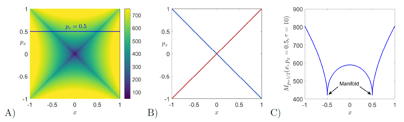
In order to support the theretical argument presented above, we provide also a numerical computation of the $p$-norm LDs in the saddle space $x-p_x$ of the linear Hamiltonian given in Eq. \eqref{eq:index1_Ham} using $p = 1/2$ and for an integration time $\tau = 10$. In Fig. fig:1 we illustrate how the method detects the stable (red) and unstable (blue) manifolds of the unstable periodic orbit at the origin, and these manifolds can be directly extracted from the ridges of the scalar field $||\nabla M_p||$. Moreover, we show in Fig. fig:1 C) that the LD scalar field is non-differentiable at the manifolds and also attains a local minimum on them, and we do so by looking at the values taken by $M_p$ along the line $p_x = 1/2$.

---

Time-dependent double well potential

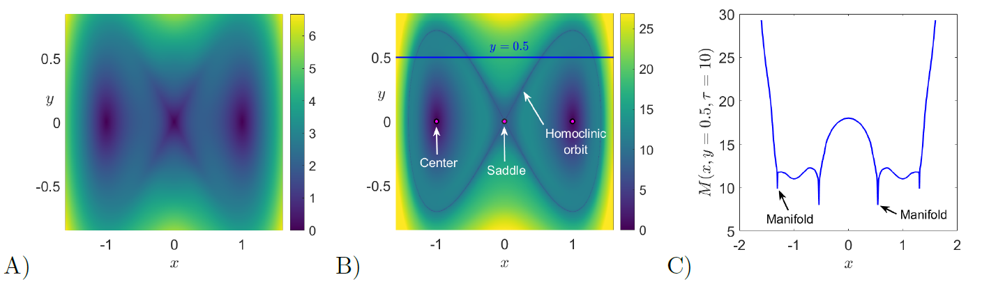
In the following example, we illustrate how the arclength definition of LDs captures the stable and unstable manifolds that determine the phase portrait of the time-dependent double well potential, commonly known in dynamical systems as the forced Duffing oscillator. The Duffing equation arises when studying the motion of a particle on a line, i.e. a one degree of freedom system, subjected to the influence of a symmetric double well potential and an external forcing. The second order ODE that describes this oscillator is given by:

\begin{equation} \ddot{x} + x^3 - x = \varepsilon f(t) \quad \Leftrightarrow \quad \begin{cases} \dot{x} = y \\ \dot{y} = x - x^3 + \varepsilon f(t) \\ \end{cases} \end{equation}

where $\varepsilon$ measures the strength of the forcing term $f(t)$, and we choose for this example a sinusoidal force $f(t) = \sin(t)$. In the autonomous case, i.e. $\varepsilon = 0$, the system has three equilibrium points: a saddle located at the origin and two diametrally opoosed centers at the points $(\pm 1,0)$. The stable and unstable manifolds that emerge from the saddle point form two homoclininc orbits in the form of a figure eight around the two center equilibria:

\begin{equation} \mathcal{W}^{s} = \mathcal{W}^{u} = \left\{(x,y) \in \mathbb{R}^2 \; \Big| \; 2y^2 + x^4 - 2x^2 = 0 \right\} \label{eq:duff_homocMani} \end{equation}

We begin by computing LDs for the unforced Duffing system using $\tau = 2$. For this small integration time, the method highlights the saddle and center fixed points, since the arclength at those points is always zero. Moreover, in this case the phase portrait still looks blurry as shown in Fig. fig:2 A), and this is a consequence of trajectories not having sufficient time to evolve in order to make distinct dynamical behaviors ditinguishable. If we now increase the integration time to $\tau = 10$, we can see in Fig. fig:2 B) that the homoclinic connection formed by the stable and unstable manifolds of the saddle point at the origin becomes clearly visible. Moreover, observe that the manifolds are located at points where the scalar values taken by LDs change abruptly. This property is demonstrated in Fig. fig:2 C), where we have depicted the value of function $M$ along the line $y = 0.5$. Notice that sharp changes in the scalar field of LDs at the manifolds are also related to local minima.

---

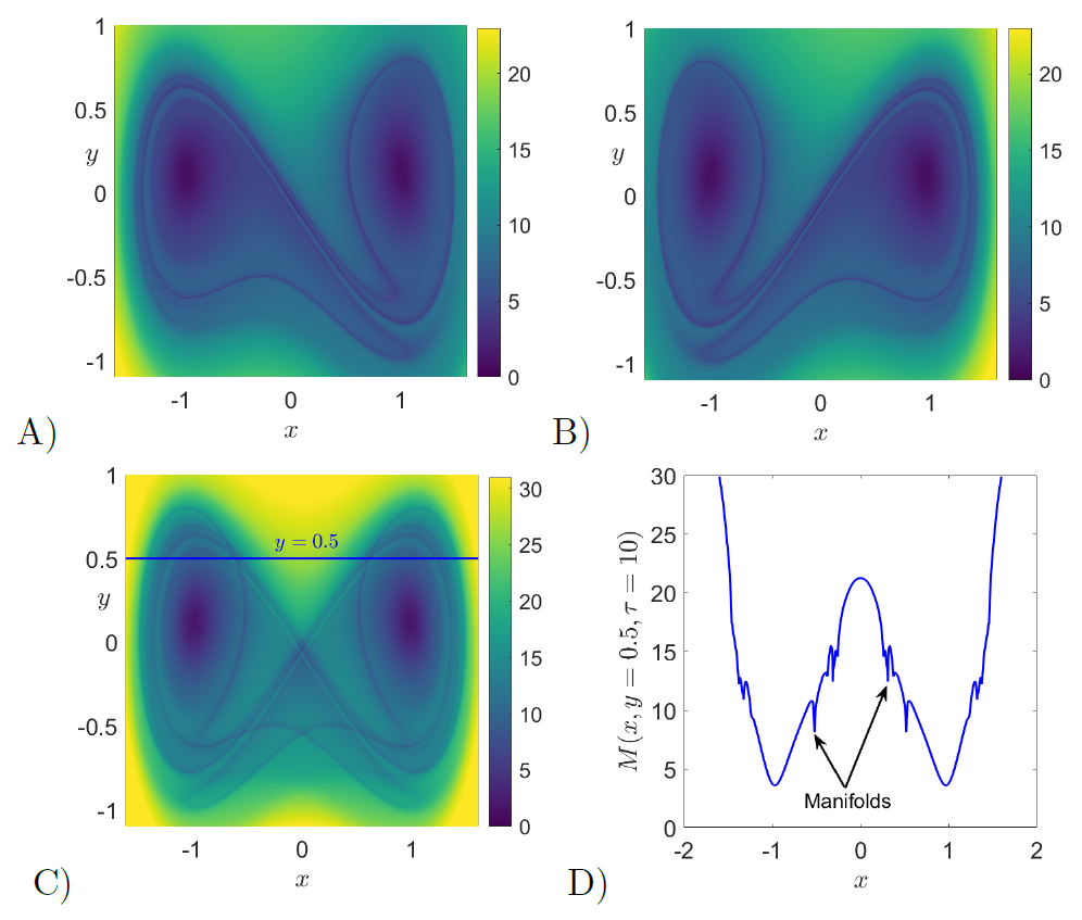
We move on to compute LDs for the forced Duffing oscillator. In this situation, the vector field is time-dependent and thus the dynamical system is nonautonomous. The consequence is that the homoclinic connection breaks up and the stable and unstable manifolds intersect, forming an intricate tangle that gives rise to chaos. We illustrate this phenomenon by computing LDs with $\tau = 10$ to reconstruct the phase portrait at the initial time $t_0 = 0$. This result is shown in Fig. fig:3 C), and we also depict the forward $(M^f)$ and backward $(M^b)$ contributions of LDs in Fig. fig:3 A) and B) respectively, demonstrating that the method can be used to recover the stable and unstable manifolds separately. Furthermore, by taking the value of LDs along the line $y = 0.5$, the location of the invariant manifolds are highlighted at points corresponding to sharp changes (and local minima) in the scalar field values of LDs.

---

Cubic potential

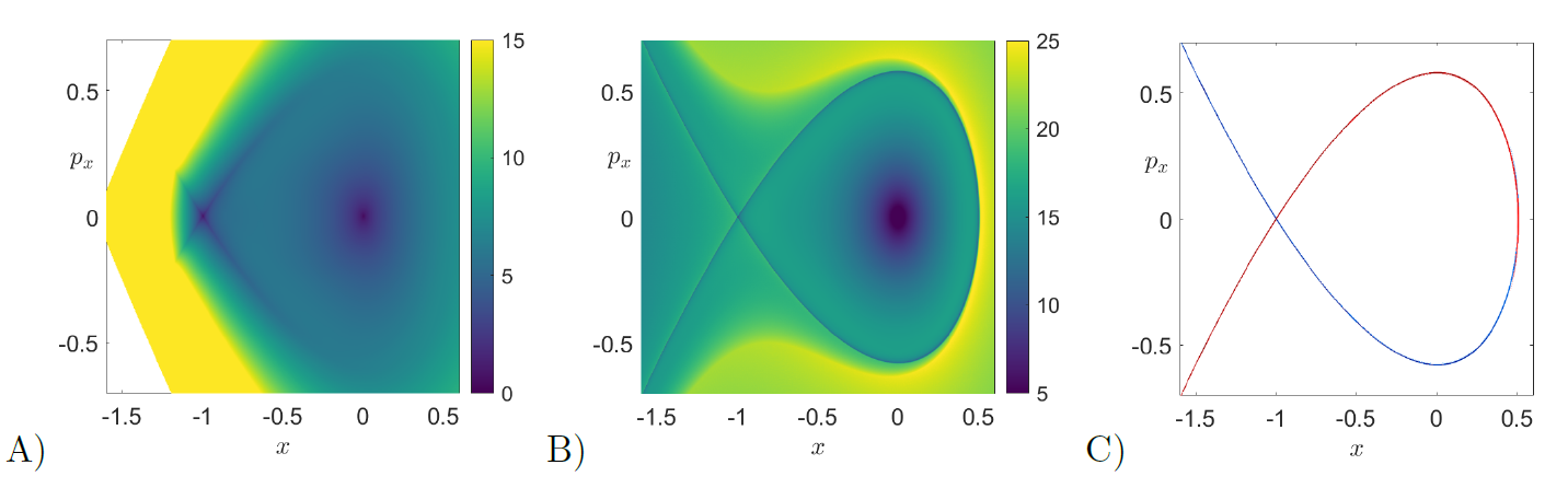
In order to illustrate the issues encountered by the fixed integration time LDs and how the variable integration approach resolves them, we apply the method to a basic one degree-of-freedom Hamiltonian known as the ''fish potential'', which is given by the formula:

\begin{equation} H = \dfrac{1}{2} p_x^2 + \dfrac{1}{2} x^2 + \dfrac{1}{3} x^3 \quad \Leftrightarrow \quad \begin{cases} \dot{x} = p_x \\ \dot{p}_{x} = - x - x^2 \end{cases} \;. \label{eq:fish_Ham} \end{equation}

This dynamical system has a saddle point at the point $(-1,0)$ from which a homoclinic orbit emerges, which surrounds the elliptic point located at the origin. By applying the $p$-norm LD with $p = 1/2$ and integrating all initial conditions for the same time $\tau = 3$ we clearly observe in Fig. fig:4 A) the problems that appear in the detection of phase space structures due to trajectories escaping to infinity in finite time. If we increase $\tau$ further, very large and NaN values of LDs completely obscure the phase portrait of the system. On the other hand, if now we use the variable integration time LDs with $\tau = 8$ and we select for the interaction region a circle of radius $r = 15$ centered at the origin, the homoclininc orbit and the equilibrium points are nicely captured. Moreover, we can extract the stable and unstable manifolds of the system from the sharp ridges in the gradient of the scalar field, due to the fact that the method is non-differentiable at the location of the manifolds.

---

Hénon-Heiles Hamiltonian

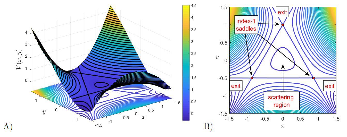
We conclude this tutorial on how to apply the method of Lagrangian descriptors to unveil the dynamical skeleton of a four-dimensional phase space by applying this tool to a hallmark Hamiltonian system of nonlinear dynamics, the H\'enon-Heiles Hamiltonian introduced in 1964 to study the motion of stars in galaxies [28]. This system is described by:

\begin{equation} H = \dfrac{1}{2} \left(p_x^2 + p_y^2\right) + \dfrac{1}{2}\left(x^2 + y^2\right) + x^2y - \dfrac{1}{3} y^3 \quad \Leftrightarrow \quad \begin{cases} \dot{x} = p_x \\ \dot{p}_{x} = - x - 2xy \\ \dot{y} = p_y \\ \dot{p}_{y} = - y - x^2 + y^2 \end{cases} \;. \label{eq:henon_system} \end{equation}

which has four equilibrium points: one minimum located at the origin and three saddle-center points at $(0,1)$ and $(\pm \sqrt{3}/2,-1/2)$. The potential energy surface is $V(x,y) = x^2/2 + y^2/2 + x^2y - y^3/3$ which has a $\pi/3$ rotational symmetry and is characterized by a central scattering region about the origin and three escape channels, see Fig. fig:5 below for details.

---

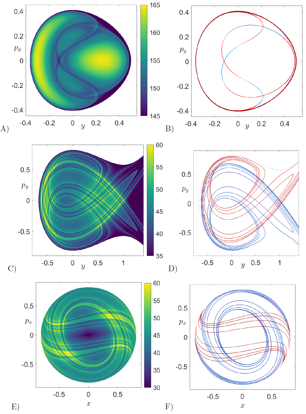
In order to analyze the phase space of the H\'enon-Heiles Hamiltonian by means of the variable integration time LDs, we fix an energy $H = H_0$ of the system and choose an interaction region $\mathcal{R}$ defined in configuration space by a circle of radius $15$ centered at the origin. For our analysis we consider the following phase space slices:

\begin{eqnarray} \mathcal{U}^{+}_{y,p_y} & = \left\{(x,y,p_x,p_y) \in \mathbb{R}^4 \;|\; H = H_0 \;,\; x = 0 \;,\; p_x > 0\right\} \\[.1cm] \mathcal{V}^{+}_{x,p_x} &= \left\{(x,y,p_x,p_y) \in \mathbb{R}^4 \;|\; H = H_0 \;,\; y = 0 \;,\; p_y > 0\right\} \label{eq:psos} \end{eqnarray}

Once we have fixed the surfaces of section (SOS) where we want to compute LDs, we select a grid of initial conditions and, after discarding those that are energetically unfeasible, we integrate the remaining conditions both forward and backward in time, and compute LDs using the definition in Eq. \eqref{eq:Mp_vt} with $p = 1/2$ along the trajectory for the whole fixed integration time or until the initial condition leaves the interaction region $\mathcal{R}$, what happens first. The result obtained when the LDs values are plotted will reveal the stable and unstable manifolds and also de KAM tori in the surface of section under consideration. Since the stable and unstable manifolds are detected at points where the LD scalar function is non-differentiable, we can directly extract them from the gradient, that is, using $||\nabla \mathcal{M}_p||$. We begin by looking at the phase space structures on the SOS $\mathcal{U}^{+}_{y,p_y}$. To do so, we fix an energy for the system $H = 1/12$, which is below that of the saddle-center equilibrium points. For that energy level, the exit channels of the PES are closed, and therefore, all trajectories are trapped in the scattering region of the central minimum at the origin. We can clearly see in Fig. fig:6 A)-B) that the computation of the $p$-norm variable integration time LDs with $p = 1/2$ using $\tau = 50$ reveals that the motion of the system is completely regular. The method nicely captures the UPO present in the central region of the PES and also its stable and unstable manifolds which form a homoclininc cnnection. In order to demonstrate how the intricate details of chaotic motion are captured by LDs, we increase the energy of the system to $H = 1/3$. This energy level is now above that of the index-1 saddles of the PES, and consequently, phase space bottlenecks open in the energy manifold allowing trajectories of the system to escape to infinity from the scattering region. When we apply LDs using $\tau = 10$ on the SOSs defined in Eq. \eqref{eq:psos}, we observe in Figs. fig:6 C)-F) that we can detect with high-fidelity the intricate homoclinic tangle formed by the stable and unstable manifolds of the UPO associated to the upper index-1 saddle of the PES. Moreover, observe that despite the issue of trajectories escaping to infinity in finite time, LDs succeed in revealing the template of geometrical phase space structures that governs transport and escape dynamics from the PES of the H\'enon-Heiles Hamiltonian system.

---

To finish this chapter we would like to mention that the method of Lagrangian descriptors has also been adapted to explore the template of geometrical structures present in the phase space of stochastic dynamical systems [29]. This achievenment clearly evidences the versatility that this mathematical technique brings to the nonlinear dynamics community. We are confident that the analysis of stochastic processes that play a crucial role in chemical reaction dynamics by means of LDs will surely help to shed light and provide new and interesting insights in the development of Chemistry. Definitely, Lagrangian descriptors has become the ultimate tool to reveal the strong bond that exists between Chemistry and Mathematics in phase space.

Implications for Reaction Dynamics

References

1. H. Poincaré, “Sur le problème des trois corps et les équations de dynamique,” Acta Mathica, vol. 13, pp. 1–270, 1890.
2. A. Coddington and N. Levinson, Theory of Ordinary Differential Equations. R.E. Krieger, 1984.
3. J. A. J. Madrid and A. M. Mancho, “Distinguished trajectories in time dependent vector fields,” Chaos, vol. 19, p. 013111, 2009.
4. C. Mendoza and A. M. Mancho, “Hidden Geometry of Ocean Flows,” Phys. Rev. Lett., vol. 105, no. 3, p. 038501, 2010.
5. A. M. Mancho, S. Wiggins, J. Curbelo, and C. Mendoza, “Lagrangian descriptors: A method for revealing phase space structures of general time dependent dynamical systems,” Communications in Nonlinear Science and Numerical Simulation, vol. 18, no. 12, pp. 3530–3557, 2013.
6. A. G. Ramos et al., “Lagrangian coherent structure assisted path planning for transoceanic autonomous underwater vehicle missions.,” Scientfic Reports, vol. 4, p. 4575, 2018.
7. V. J. Garcia-Garrido, A. Ramos, A. M. Mancho, J. Coca, and S. Wiggins, “A dynamical systems perspective for a real-time response to a marine oil spill.,” Marine Pollution Bulletin., pp. 1–10, 2016.
8. A. de la Cámara, A. M. Mancho, K. Ide, E. Serrano, and C. R. Mechoso, “Routes of transport across the Antarctic polar vortex in the southern spring.,” J. Atmos. Sci., vol. 69, no. 2, pp. 753–767, 2012.
9. A. de la Cámara, R. Mechoso, A. M. Mancho, E. Serrano, and K. Ide., “Isentropic transport within the Antarctic polar night vortex: Rossby wave breaking evidence and Lagrangian structures.,” J. Atmos. Sci., vol. 70, pp. 2982–3001, 2013.
10. J. Curbelo, C. R. Mechoso, A. M. Mancho, and S. Wiggins, “Lagrangian study of the final warming in the southern stratosphere during 2002: Part I. The vortex splitting at upper levels,” Climate Dynamics, vol. 53, no. 5, pp. 2779–2792, 2019.
11. J. Curbelo, C. R. Mechoso, A. M. Mancho, and S. Wiggins, “Lagrangian study of the final warming in the southern stratosphere during 2002: Part II. 3D structure,” Climate Dynamics, vol. 53, no. 3, pp. 1277–1286, 2019.
12. G. T. Craven and R. Hernandez, “Lagrangian descriptors of thermalized transition states on time-varying energy surfaces,” Physical review letters, vol. 115, no. 14, p. 148301, 2015.
13. G. T. Craven and R. Hernandez, “Deconstructing field-induced ketene isomerization through Lagrangian descriptors,” Physical Chemistry Chemical Physics, vol. 18, no. 5, pp. 4008–4018, 2016.
14. G. T. Craven, A. Junginger, and R. Hernandez, “Lagrangian descriptors of driven chemical reaction manifolds,” Physical Review E, vol. 96, no. 2, p. 022222, 2017.
15. F. Revuelta, R. M. Benito, and F. Borondo, “Unveiling the chaotic structure in phase space of molecular systems using Lagrangian descriptors,” Physical Review E, vol. 99, no. 3, p. 032221, 2019.
16. W.-L. Chien, H. Rising, and J. M. Ottino, “Laminar mixing and chaotic mixing in several cavity flows,” Journal of Fluid Mechanics, vol. 170, pp. 355–377, 1986.
17. A. S. Demian and S. Wiggins, “Detection of Periodic Orbits in Hamiltonian Systems Using Lagrangian Descriptors,” International Journal of Bifurcation and Chaos, vol. 27, no. 14, p. 1750225, 2017.
18. S. Naik, V. J. García-Garrido, and S. Wiggins, “Finding NHIM: Identifying high dimensional phase space structures in reaction dynamics using Lagrangian descriptors,” Communications in Nonlinear Science and Numerical Simulation, vol. 79, p. 104907, 2019.
19. S. Naik and S. Wiggins, “Finding normally hyperbolic invariant manifolds in two and three degrees of freedom with Hénon-Heiles type potential,” Phys. Rev. E, vol. 100, no. 2, p. 022204, 2019.
20. V. J. García-Garrido, S. Naik, and S. Wiggins, “Tilting and Squeezing: Phase space geometry of Hamiltonian saddle-node bifurcation and its influence on chemical reaction dynamics,” arXiv preprint:1907.03322 (\it Under Review), 2019.
21. C. Lopesino, F. Balibrea-Iniesta, V. J. García-Garrido, S. Wiggins, and A. M. Mancho, “A Theoretical Framework for Lagrangian Descriptors,” International Journal of Bifurcation and Chaos, vol. 27, no. 01, p. 1730001, 2017.
22. M. Feldmaier et al., “Invariant Manifolds and Rate Constants in Driven Chemical Reactions,” The Journal of Physical Chemistry B, vol. 123, no. 9, pp. 2070–2086, 2019.
23. A. Junginger, L. Duvenbeck, M. Feldmaier, J. Main, G. Wunner, and R. Hernandez, “Chemical dynamics between wells across a time-dependent barrier: Self-similarity in the Lagrangian descriptor and reactive basins,” The Journal of chemical physics, vol. 147, no. 6, p. 064101, 2017.
24. I. Mezic and S. Wiggins, “A method for visualization of invariant sets of dynamical systems based on the ergodic partition,” Chaos, vol. 9, no. 1, pp. 213–218, 1999.
25. A. Weinstein, “Normal modes for nonlinear Hamiltonian systems,” Inventiones mathematicae, vol. 20, no. 1, pp. 47–57, 1973.
26. J. Moser, “Periodic orbits near an equilibrium and a theorem by Alan Weinstein,” Communications on Pure and Applied Mathematics, vol. 29, no. 6, pp. 727–747, 1976.
27. P. H. Rabinowitz, “Periodic solutions of Hamiltonian systems: a survey,” SIAM J. Math. Anal., vol. 13, no. 3, pp. 343–352, 1982.
28. M. Hénon and C. Heiles, “The Applicability of the Third Integral of Motion: Some Numerical Experiments,” Astronom. J., vol. 69, pp. 73–79, 1964.
29. F. Balibrea-Iniesta, C. Lopesino, S. Wiggins, and A. M. Mancho, “Lagrangian Descriptors for Stochastic Differential Equations: A Tool for Revealing the Phase Portrait of Stochastic Dynamical Systems,” International Journal of Bifurcation and Chaos, vol. 26, no. 13, p. 1630036, 2016.