Influence of Mass and Energy Surface Geometry in Chesnavich's Model

Introduction

Following recent developments in the understanding of the roaming mechanism in molecular dynamics (missing reference), the results of Heazlewood et al. [1] on roaming being the dominant mechanism for acetaldehyde photodissociation triggered the following question: Can some of the standard parameter values in Chesnavich's CH+4 model [2] be altered so that it admits roaming as the dominant form of dissociation? It is well known that roaming plays a minor role in the dissociation of Formaldehyde[3]. Since acetaldehyde dissociates into CH4+CO, one of the obvious differences in the dissociation of Formaldehyde into H2+CO is the mass ratio of the products. Therefore we investigate the influence of various masses of the free atom on roaming in Chesnavich's CH+4 model. Furthermore we consider different values of parameter a, the coupling parameter of the angular and radial degrees of freedom in Chesnavich's potential, and deduce its impact on roaming. Physically speaking, a controls the strength of the short range anisotropy of the CH+3 molecule and its precise role in the potential is discussed in Section sec:2.

Chesnavich's CH+4 model [2] is a phenomenological 2 degree of freedom model introduced that was introduced to study the transition from vibrational reactants to rotational products in the presence of multiple transition states. We use it to study the first stage of roaming, where a hydrogen atom separates from the rigid CH+3 molecule and instead of dissociating, it roams in a region of nearly constant potential only to return to the molecule without forming a bond. The process of intramolecular abstraction and subsequent dissociation requires both H atoms to be mobile and thus requires at least 4 degrees of freedom. At the moment no tools for a qualitative dynamical study that would explain roaming in its entirety in 4 degrees of freedom have been developed.

Roaming

Roaming was discovered in the study of photodissociation of formaldehyde [3] (H2CO) and explained the unusual energy distribution between H2 and CO experimentally observed previously [4]. Since then roaming was reported in a number of other molecules (missing reference). Initial states of roaming resemble radical dissociation, when a single H atom escapes from HCO by breaking a single covalent bond and immediately dissociates. Instead of dissociating, the free hydrogen 'roams' around a flat monotonic region of the potential near HCO and returns to the molecule to abstract the remaining hydrogen. Ultimately, the products of this dissociation are identical to the products of molecular dissociation. While molecular dissociation requires the system to pass over a potential saddle, no saddle is involved in roaming. Consequently the distribution of energy between the products can differ significantly. Following a study [5] of H2CO and CH3CHO it was established that regardless of similarity of products, roaming is actually closer to radical dissociation than to molecular dissociation and further evidence was published subsequently [6].

In light of developments following a phase space approach to chemical reaction dynamics [7], [8], [9], we employ the definition of roaming introduced in Ref. . This definition considers the number of intersections of a trajectory with a dynamically justified dividing surface and thereby accounts for the influence of various phase space structures. The dividing surface is constructed using an unstable periodic orbit that is not associated with any potential saddle. It was shown [10] how invariant manifolds of unstable periodic orbits convey trajectories between two potential wells in what is called a 'shepherding mechanism'. The exact phase space structure, an intersection of invariant manifolds of unstable periodic orbits, responsible for roaming was since identified (missing reference). The key to understanding roaming follows from the use of toric surfaces of section [11], [12], [13] to study invariant manifolds.

Development of the Problem

We study the system in a polar centre of mass frame, where r is the distance of the mobile H atom from the centre of mass of the system in Å and θ is the angle describing the relative orientation of H and CH+3 in radians. The momenta pr and pθ are cannonically conjugate to r and θ respectively.

The model we study is defined by the Hamiltonian

H(r,θ,pr,pθ)=12μp2r+12p2θ(1I+1μr2)+U(r,θ),

where μ=mCH3mHmCH3+mH, with mH=1.007825 u and mCH3=12.0 u, is the reduced mass of the system, and I=2.373409 uÅ2 is the moment of inertia of the rigid body CH+3. Chesnavich's potential U(r,θ) has the form

U(r,θ)=UCH(r)+Ucoup(r,θ),

and it is the sum of radial long range potential UCH and short range "hindered rotor" potential Ucoup, that represents the anisotropy [2], [14] of the rigid molecule CH+3. We use the standard definition of UCH and Ucoup and standard parameter values as suggested by Chesnavich [2] and used in recent publications (missing reference), namely

UCH(r)=Dec1−6(2(3−c2)ec1(1−x)−(4c2−c1c2+c1)x−6−(c1−6)c2x−4),

where x=rre, De=47 kcal/mol, re=1.1 Å, c1=7.37 and c2=1.61, and

Ucoup(r,θ)=Uee−a(r−re)22(1−cos2θ),

where Ue=55 kcal/mol. The parameter a (in Å−2) influences the value of r at which the transition from vibration to rotation occurs, for example a=1 represents a late transition (missing reference) and a=4 an early transition [15]. In this chapter we shall explore all values of a that may be relevant to roaming.

The total energy H(r,θ,pr,pθ)=E is given in kcal/mol with respect to the dissociation energy 0.

We introduce the potential in more detail and explain the role of the parameter a is Section sec:2{reference-type="ref" reference="sec:potential"}. Subsequently we give an overview of roaming up to date in Section sec:1, we explain how phase space structures influence the dynamics in Section sec:3 and focus on how these structures cause roaming in sec:4.

To study the dependence of roaming on the mass of the free atom, we replace the free H atom by a atom of mass m, so that the reduced mass of the system is μm=mCH3mmCH3+m and the Hamiltonian then is

Hm(r,θ,pr,pθ)=12μmp2r+12p2θ(1I+1μmr2)+U(r,θ).

In this work we consider m<mCH3, since the free atom is usually the lighter of the two dissociated products. For comparison, the free atom would have to weight m=8.57 to be in the same proportion as in acetaldehyde.

Since m is only present in the kinetic part of the Hamiltonian (Equation (5)), its influence cannot be seen in configuration space. We explain how variations in mass of the free atom influence the system, phase space structures and roaming in different parts of phase space in Sections sec:5, sec:6 and sec:7.

The phase space structures that enable us to study dynamics in phase space are normally hyperbolic invariant manifolds (NHIMs) and the corresponding stable and unstable invariant manifolds. We build upon the understanding of the role of NHIMs and invariant manifolds in governing dynamics as described in Refs. in great detail.

Role of the coupling parameter (a)

The potential U(r,θ) as defined by Equations (2), (3) and (4), has the following characteristics:

• potential wells near θ=0 and θ=π representing the two isomers of CH+4,

• areas of high potential near θ=π2 and θ=3π2 creating a potential barrier between the two wells,

• an area where the potential is monotonic and nearly constant due to U(r,θ)∈o(r−4) as r→∞, representing the dissociated state.

Note that due to the rotational symmetry U(r,θ)=U(r,θ+π) and reflectional symmetry U(r,θ)=U(r,−θ) of U that follows from the anisotropic term Ucoup in Equation (4)), the wells and areas of high potential are symmetric.

All of the characteristics listed above can be derived from the critical points of U(r,θ). Table tab:1 shows critical points of U for 0≤θ<π, while symmetric counterparts exist in −π≤θ<0. We denote critical points by q, the subscript indicates the index of the saddle and the superscript indicates the half plane in which the critical point lies: + for 0≤θ<π, − for −π≤θ<0.

Energy (kcal mol−1)	r (Å)	θ (radians)	Significance	Label
−47	1.1	0	potential well	q+0
>0	<1.1	π/2	isomerisation saddle	q+1
>0	>1.1	π/2	local maximum	q+2
<0	>1.1	π/2	isomerisation saddle	˜q+1

---

We remark that q+1 and q+2 are energetically inaccessible at energies considered in this work. Four more critical points q−0, q−1, q−2 and ˜q−1 are related to the ones above by symmetry. The location of the critical points in configuration space can be seen in Figure fig:1 for a=1,3,6,8.

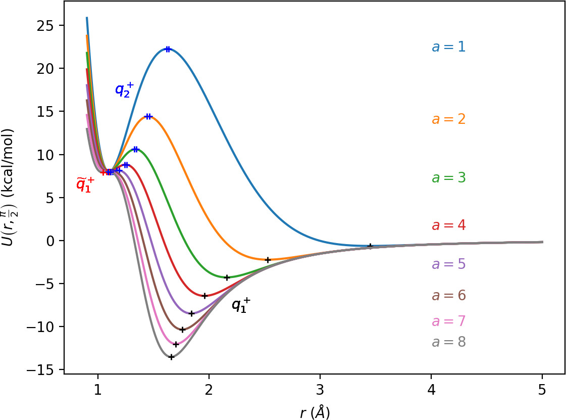
The coupling term Ucoup through which a influences the potential, vanishes around θ=0 and θ=π and is maximal around θ=±π2. Therefore variations of a leave most of the well unaffected, while the potential maxima and associated critical points vary significantly. Figure fig:2 illustrates how the potential barrier between the wells recedes with increasing a. The figure also shows how q+1, q+2 and ˜q+1 are affected by a, note the decrease of energy of q+1. When considered in context of the contour plots in Figure fig:1, for a=6 and larger the wells merge into one from an energetic perspective, but dynamically remain distinct.

---

---

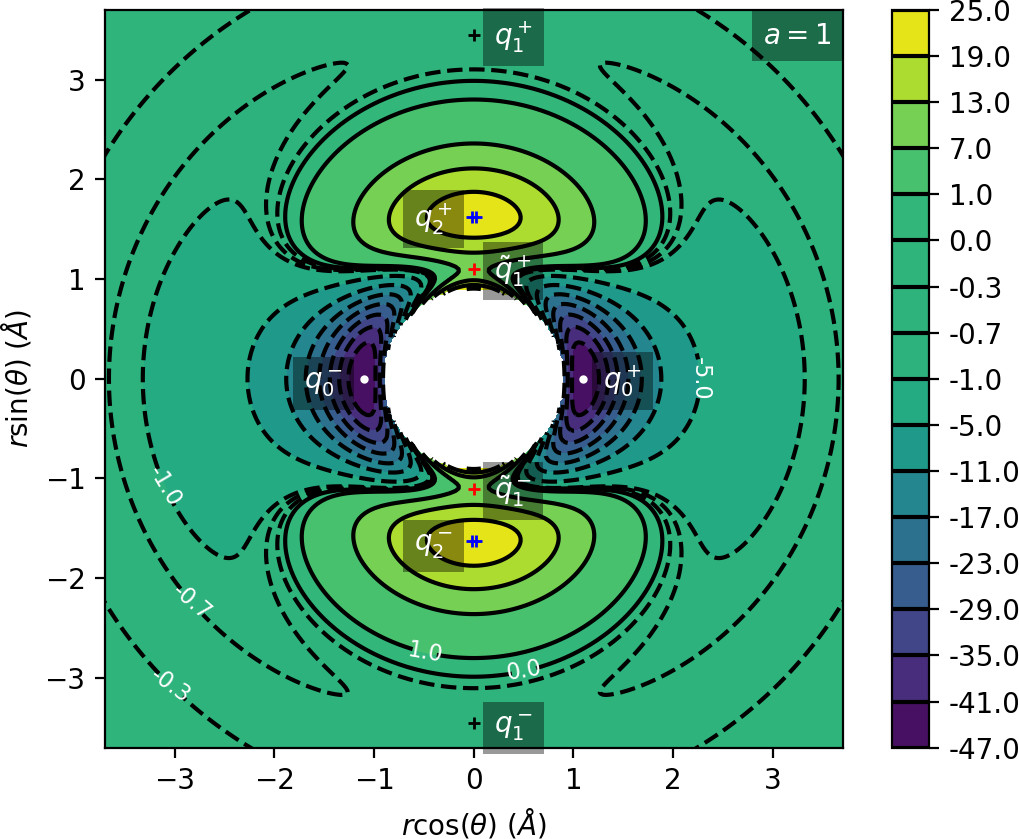
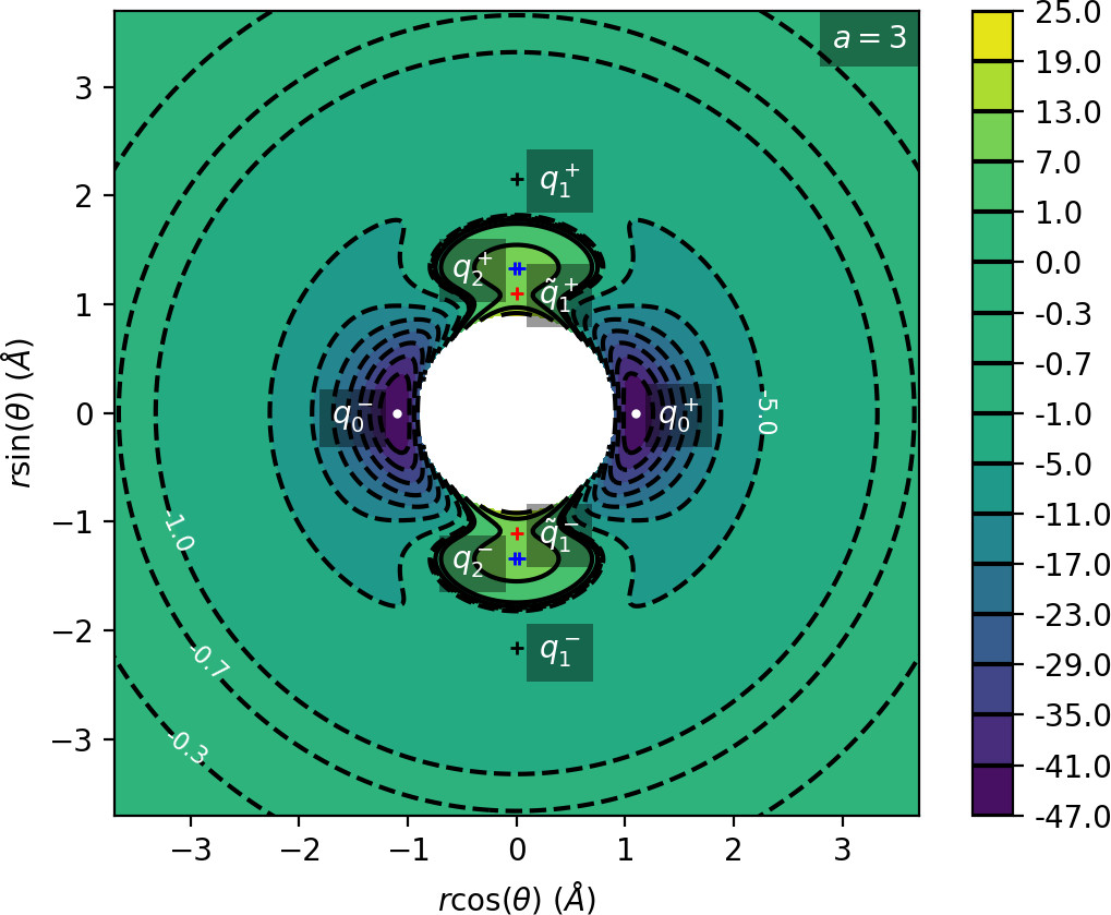
Due to the exponential decay of the anisotropic term Ucoup and the o(r−4) decay of U as a whole, the area of flat potential that can be seen in Figures fig:1 and fig:2 remains unchanged. In this area U is negative, monotonic in r, very close to zero and certainly has no saddles.

Apart from different values of the potential, the wells also differ from the area of flat potential dynamically. In the potential well trajectories vibrate, i.e. oscillate in the angular direction, as they are bounded by the two areas of high potential. Outside of the wells, especially in the flat area, the absence of potential barriers enables unlimited movement in the angular direction that is manifested in trajectories completing full rotations around the centre of mass. The transition from one type of dynamics to the other depends heavily on the size and height of the areas of high potential that is influenced by a as described above.

Revealing the Phase Space Structures

There are three important families of periodic orbits (missing reference) in Chesnavich's CH+4 model. By family of periodic orbits we mean a continuum of periodic orbits parametrised by energy, so that each family contains two orbits related by (reflectional) symmetry for a given E. We will refer to these orbits as the inner (Γi), middle (Γa) and outer (Γo) periodic orbit based on the radii of the orbits and their significance in dissociation. For a given E, the middle and outer families consist of two orbits with the same configuration space projections but opposite orientation, one with pθ>0 and one with pθ<0, hence clearly distinct in phase space. In a configuration space projection these orbits rotate counterclockwise and clockwise respectively. The inner family consists of two orbits, one on the edge of each potential well. In the following, statements regarding one of the orbits of a family automatically hold for the other one due to symmetry. If we only refer to one orbit, we refer to Γa and Γo with pθ>0 and Γi oscillating around θ=0.

Configuration space projections are shown in Figure fig:3. Note that none of these families is associated with a saddle point on the potential energy surface.

---

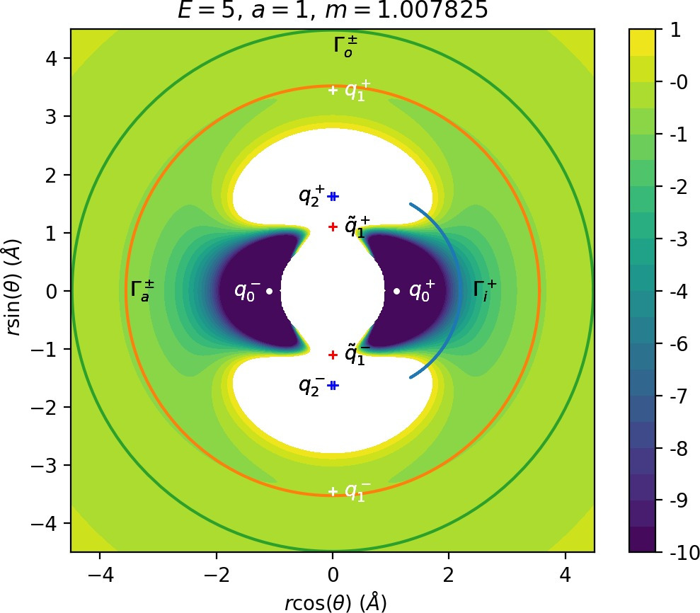
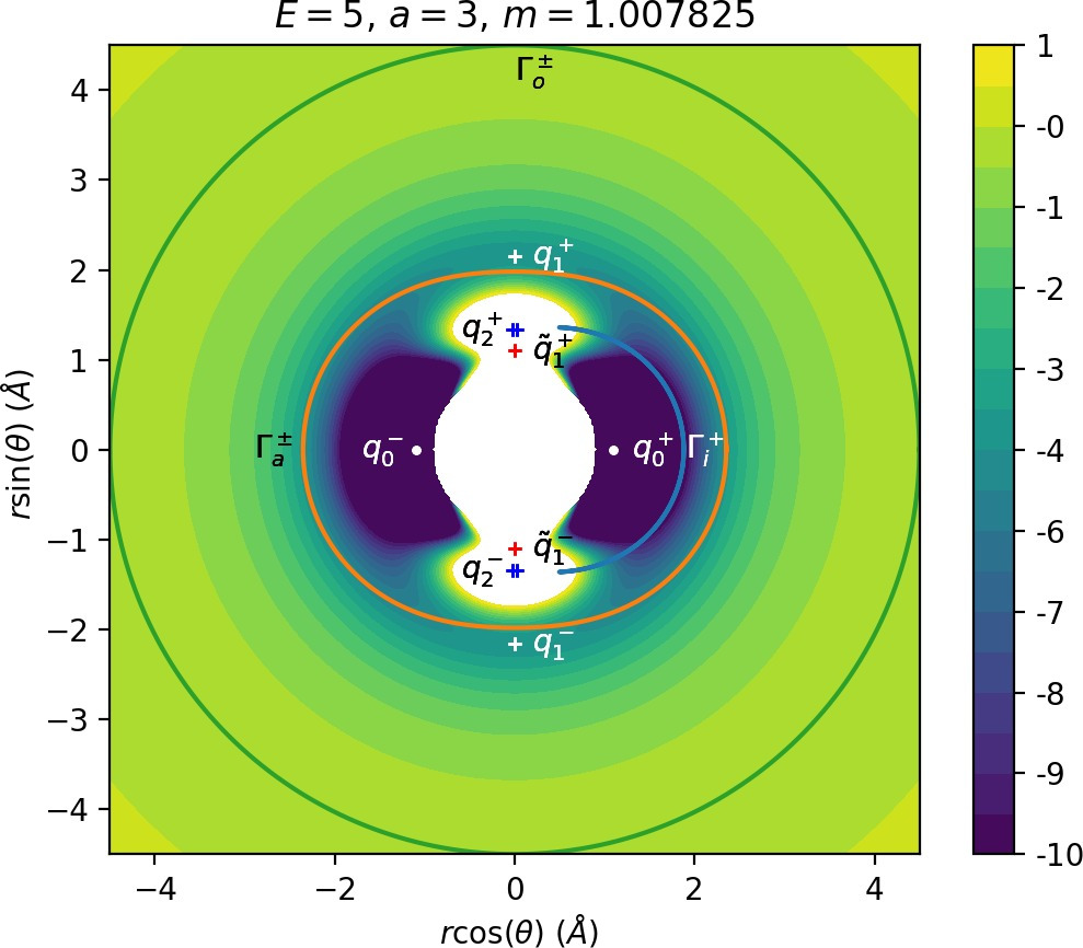
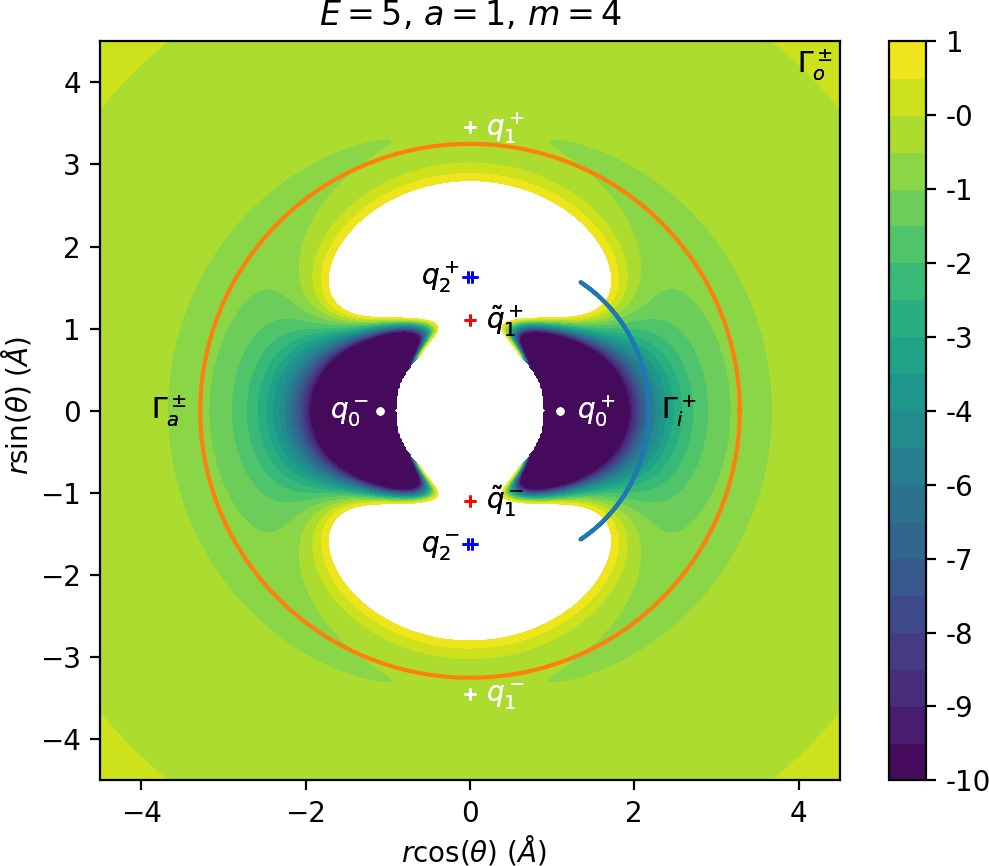
The family of outer periodic orbits Γo is proven (missing reference) to exist due to a centrifugal barrier for a class of systems including the one considered here. It was also shown that the orbits in this family are unstable. States of the system beyond the outer orbits correspond to dissociated states CH+3+H. Orbits of this family are therefore the outer boundary of the roaming region [16]. We prefer to use the more general term interaction region as the phase space structures responsible for roaming and isomerisation among trajectories that leave the well, also arbitrate whether incoming trajectories originating at r=∞ react (reach the well) or not. In the context of transition state theory, this region is sometimes also called the collision complex.

The potential wells represent the region where the CH+4 molecule is in a stable configuration and orbits of the inner family Γi naturally delimit this region. All inner periodic orbits are unstable and form the inner boundary of the interaction region.

Inside the interaction region lies the family of middle orbits, which are crucial in the definition of roaming. These orbits are unstable for small positive energies (E<2.72 for a=1 and m=mH) and stable after a period doubling bifurcation involving a family denoted sometimes by FR12 [16], [15] or Γb (missing reference) that is of no further importance. The exact energy of the period doubling bifurcation varies with m and a, but for m=mH and a=1 is at approximately E=2.72. The family is also subject to bifurcations at negative energies, but these are not relevant for roaming.

The definition of roaming as introduced in Ref. requires us to construct a dividing surface in phase space based on the configuration space projection of Γa. We shall denote the dividing surface associated with Γa as DSa. For a given energy E, DSa consists of all points (r,θ,pr,pθ) on the energy surface Hm(r,θ,pr,pθ)=E, such that (r,θ) is a point on the configuration space projection of Γa.

It is known that a spherical dividing surface may in the neighbourhood of an index-1 saddle bifurcate into a torus [11], [12] and it was recognised [13] that dividing surfaces constructed using periodic orbits that rotate such as DSa, as opposed to vibrate, are tori. In addition, if Γa is unstable, then DSa does not admit local recrossings.

Indeed one can see that for every point (rΓa,θΓa) on the configuration space projection of Γa, the corresponding phase space structure is a circle implicitly defined by (Equation (5)) as E−U(rΓa,θΓa)=12μmp2r+12p2θ(1I+1μmr2).

Note that the radius of the circle never vanishes along Γa as the kinetic energy never vanishes along Γa.

A trajectory is considered a roaming trajectory if it originates in the potential well and crosses DSa at least three times before dissociating. If a trajectory crosses DSa an even number of times and enters either one of the potential wells, it is an isomerisation trajectory.

Roaming can be reformulated as a transport problem (missing reference) in the following manner. Let DSi and DSo be defined using Γi and Γo analogously to DSa. It is well known that a dividing surface associated with a periodic orbit that reaches two equipotentials, such as Γi, is a sphere. Using reasoning similar to the above one can see, that because the kinetic energy along Γi vanishes when it reaches the equipotentials, DSi consists of circles except for the poles which are points, thus a sphere. Γi, being the equator of this sphere, divides it into two hemispheres with unidirectional flux - trajectories leaving the well cross the outward hemisphere while trajectories entering the well cross the inward hemisphere.

DSa and DSo are tori, but they too can be divided into two parts of unidirectional flux. This can be easily seen on DSo, but a similar argument applies to DSa. Since Γo has a constant radius and pr=0, the two orbits are characterised by p2θ being maximal for the given energy along the orbit. Any trajectory crossing DSo must therefore have pr≠0. All trajectories with pr>0 cross the outward annulus of DSo bounded by the two orbits Γo, while all with pr<0 cross the inward annulus and enter the interaction region.

Note that because dividing surfaces divide the energy surface into two separate partitions, the dividing surfaces defined above have the following roles. Since Γi lies on the edge of the potential well, the role of DSi is to divide the the energy surface region associated with the potential well from the rest of the energy surface. Every trajectory that enters or exists the well must cross DSi. Similarly, DSo is used to divide the dissociated states from the rest of the energy surface and every trajectory going from one part of the energy surface into the other must cross DSo. DSa divides the the energy surface interaction region between DSi and DSo into two, but neither of the two partitions bears a relevant meaning. The definition of roaming is the sole purpose of this surface in this investigation.

Implications for Reaction Dynamics

We can formulate dissociation as a problem of transport of trajectories between dividing surfaces in the following manner. By definition, trajectories that leave the well must cross the outward hemisphere of DSi. Trajectories that leave the interaction region (dissociate), cross the outward annulus of DSo. Dissociation is therefore a question of how trajectories from the outward hemisphere of DSi reach the outward annulus of DSo.

In the process of being transported from DSi to DSo, dissociating trajectories originating must cross the outward annulus of DSa. Roaming trajectories cross the torus DSa at least three times, first the outward annulus and then alternately the inward and the outward annulus. It should be noted that trajectories originating in either of the wells have to cross the outward annulus of DSa before they can reach its inward annulus. Similarly trajectories going from the inward annulus of DSa to the outward annulus of DSo must cross the outward annulus of DSa. Therefore trajectories that originate in the well and cross the inward annulus of DSa before dissociating are roaming trajectories.

The role of phase space structures in reaction dynamics has been explained on many occasions [7], [8], [9]. Dividing surfaces as defined above can be shown to be the surfaces of minimal flux [9] and therefore sit in the narrowest part of the bottleneck, be it a sphere such as DSi or a torus such as DSa and DSo. Structures that convey trajectories across such a bottleneck were identified to be stable and unstable invariant manifolds of the unstable periodic orbit. These invariant manifolds have a cylindrical structure and form a barrier between trajectories that are lead through the bottleneck (inside) and those are not (outside).

For each unstable orbit Γ, there are two branches of stable invariant manifold, i.e. manifolds consisting of a continuum of trajectories that are asymptotic to the orbit in forward time, and two branches of unstable invariant manifold, asymptotic in backward time. We shall denote the invariant manifolds of Γ by WΓ, we distinguish stable and unstable by a superscript, WsΓ and WuΓ, and if we refer to an individual branch, we add a + or − to the superscript to indicate, whether the branch leaves the neighbourhood of Γ to the r>rΓ side (+) or to the r<rΓ side (−).

The precise cylindrical structure of the manifold reflects the geometry of the corresponding periodic orbit in a similar way as it is reflected by the corresponding dividing surface. Manifolds WΓi are spherical cylinders, whereas WΓa and WΓo are toric cylinders. The different geometries can be understood from a phase space perspective.

For any fixed energy, Γi is a (topological) circle with its center, due to symmetry of the system, on the ray θ=0, pr=pθ=0. This property is passed on to all four branches of WΓi, these too are always centered at/symmetric with respect to θ=0, pr=pθ=0, no matter how heavily they are deformed by the flow which is smooth.

In contrast, WΓa and WΓo are centered at r=0, just like the corresponding orbits Γa and Γo. This property is independent of energy.

All of this is a consequence of the local energy surface geometry that is not uniform throughout the energy surface and can be observed as qualitatively different forms of dynamics - vibration and rotation.

Phase space structures responsible for roaming

We study invariant manifolds and their intersections on a surface of section, namely on an accurate approximation of the outward annulus of DSa. Both annuli of DSa are transversal to the flow and are bounded by Γa. Suppose the configuration space projection of Γa can be parametrised using the function ˉr(θ) as (ˉr(θ),θ) and define

ρ(r,θ)=r−ˉr(θ).

Clearly Γa is then given by ρ(r,θ)=0,

and the outward annulus of DSa is defined by all points (r,θ,pr,pθ) on the energy surface, such that ρ(r,θ)=0,˙ρ(r,θ)>0. Note that ˙ρ(r,θ)>0 is not equivalent to ˙r>0.

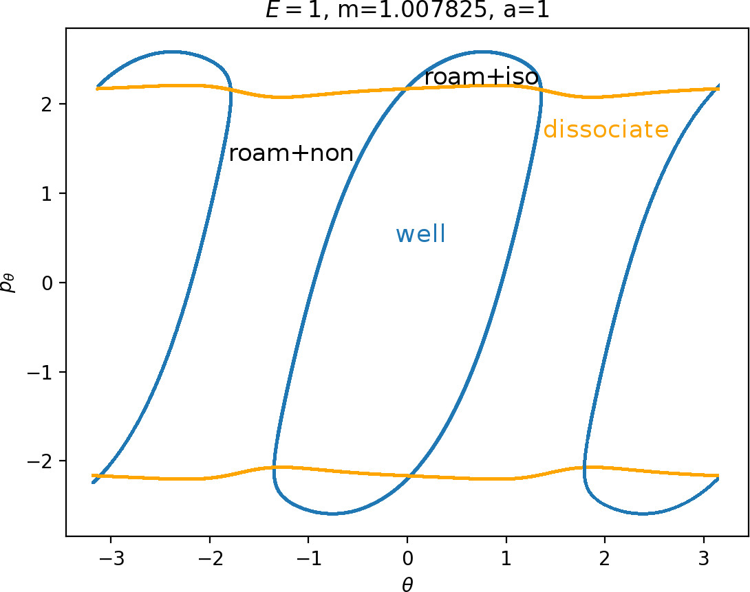
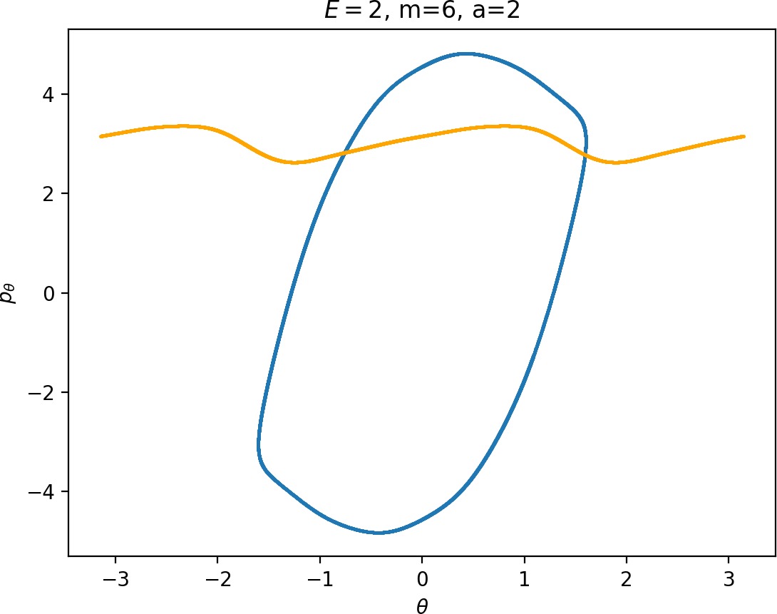
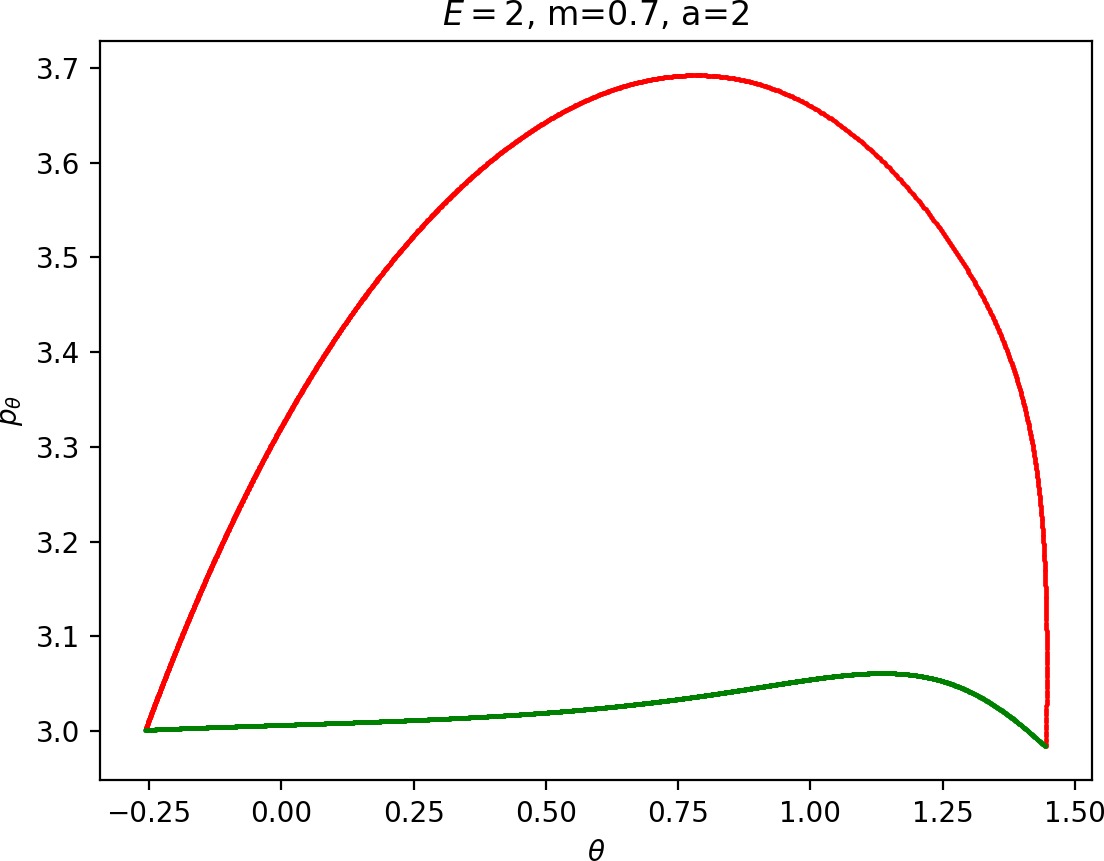
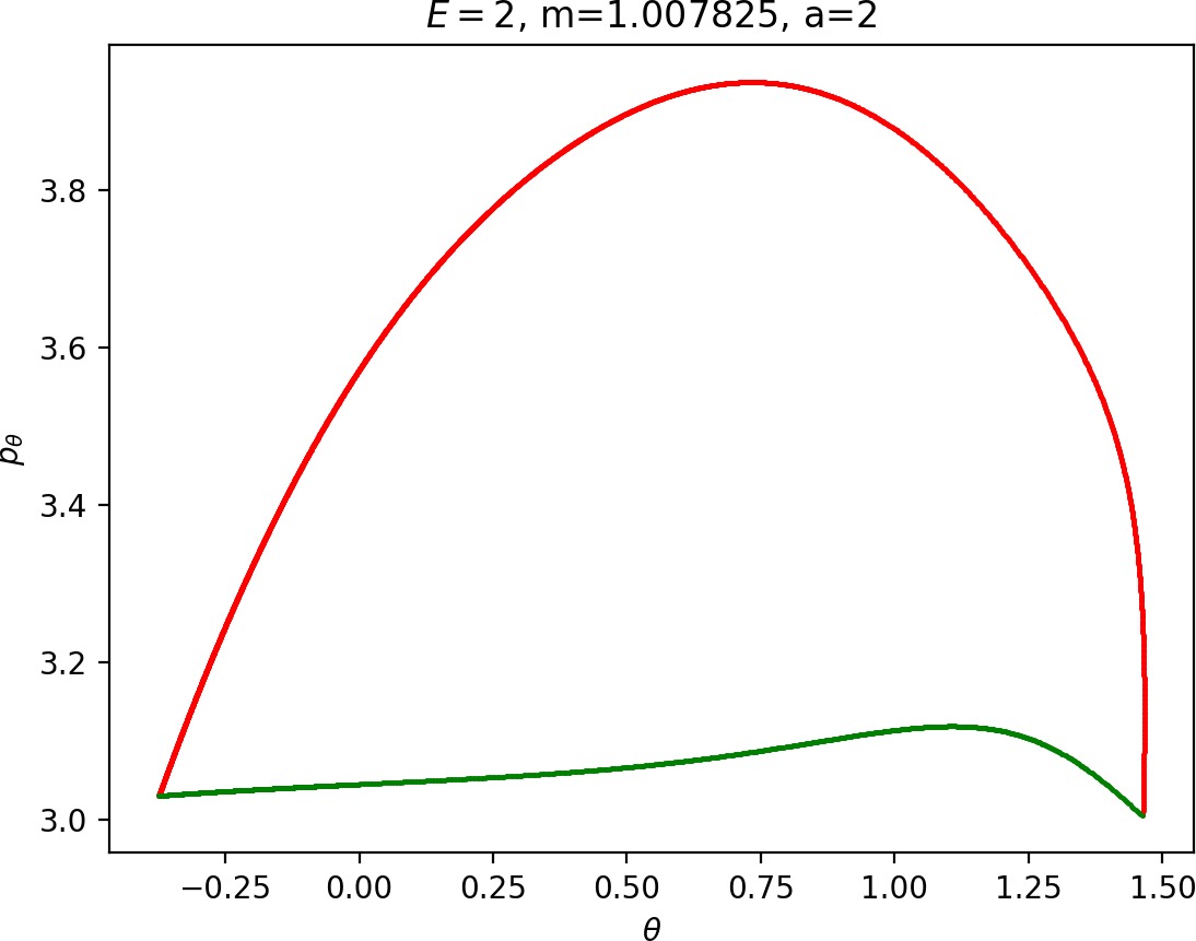
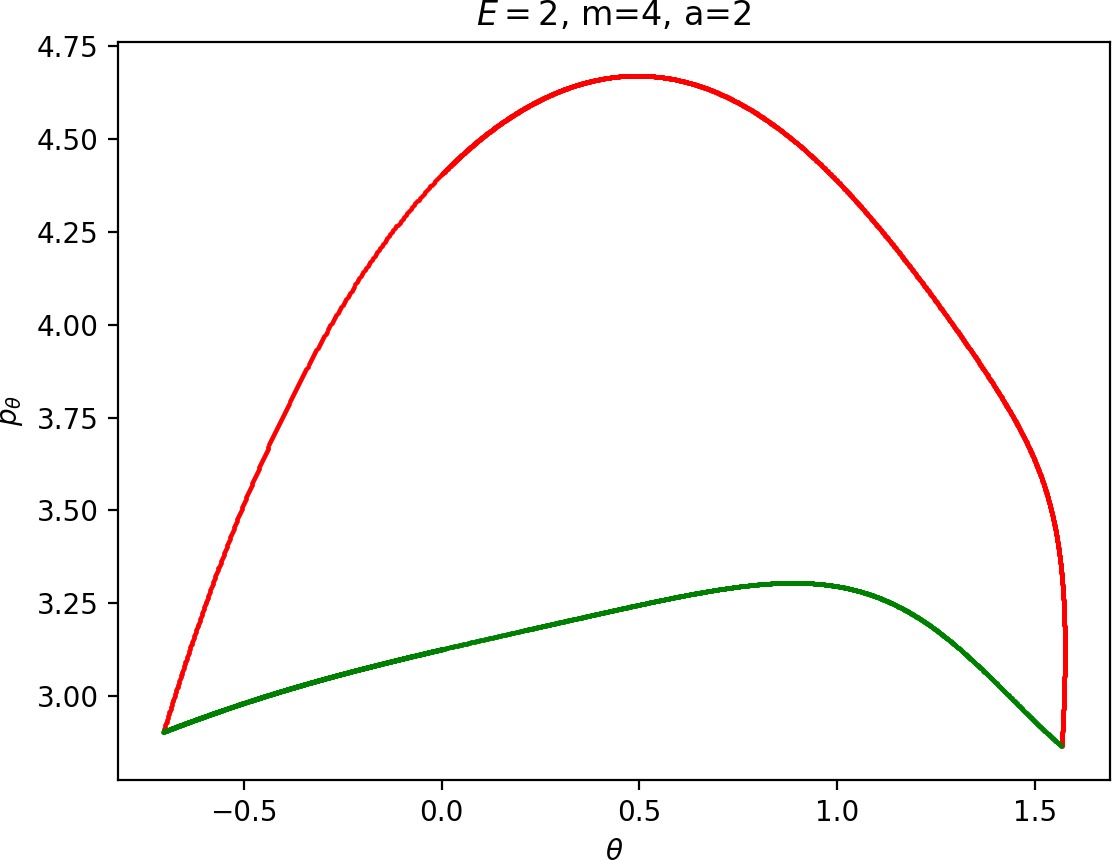
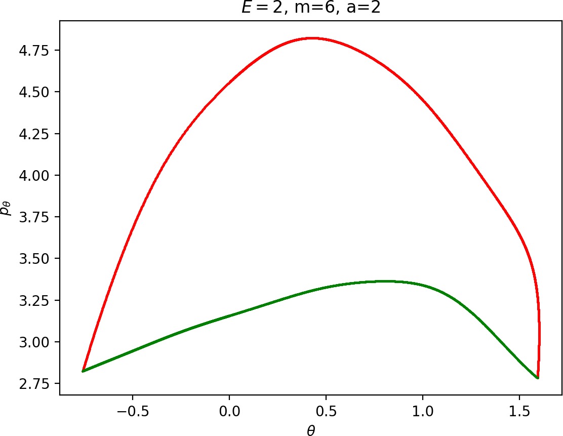
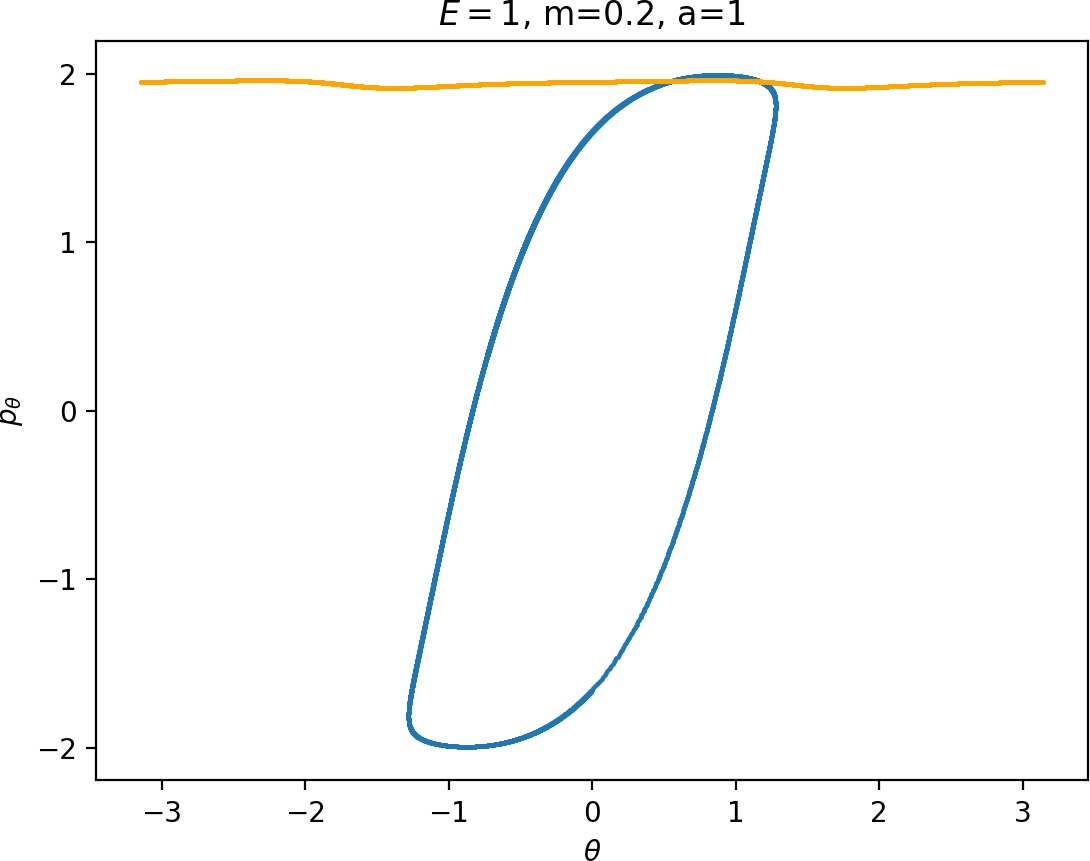
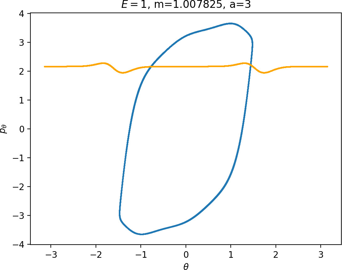
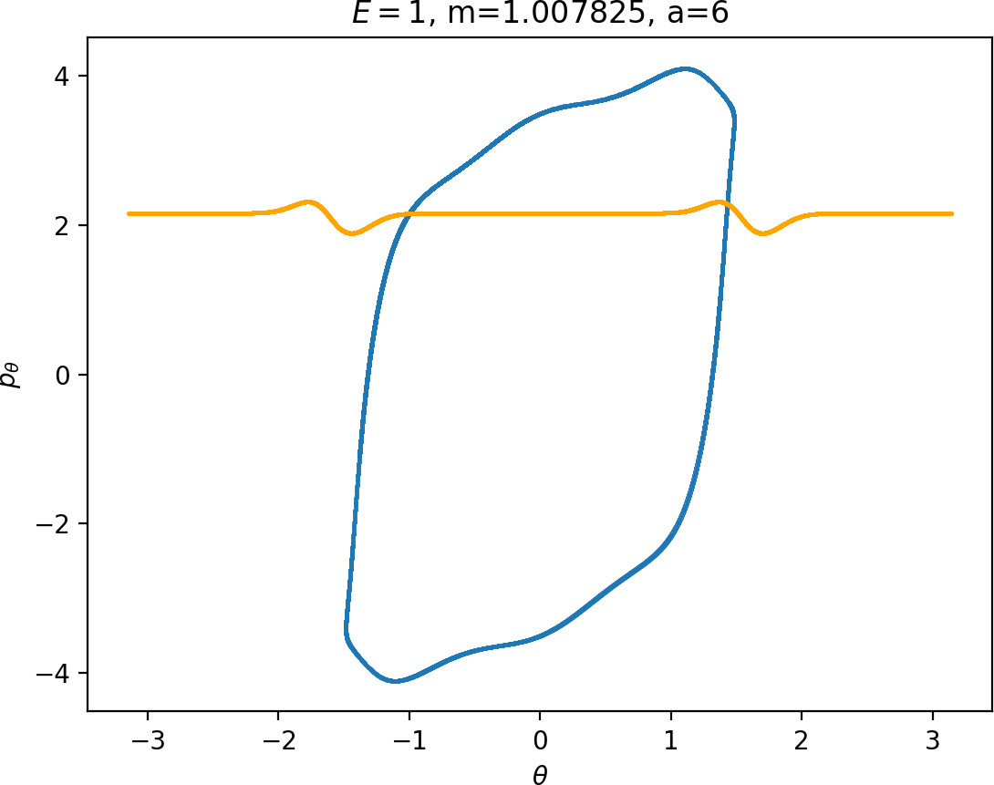
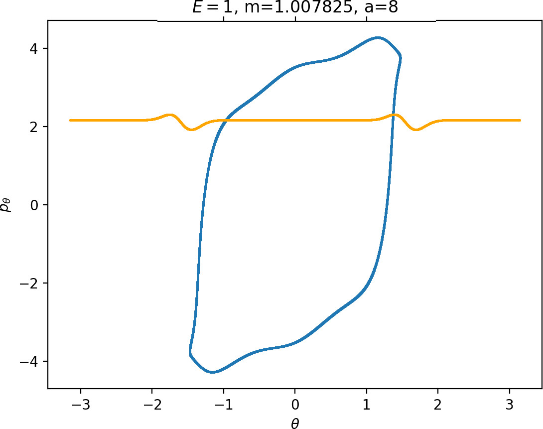
Most notably, we are interested in the interaction between Wu+Γi, the manifold guiding trajectories that leave the potential well into the interaction region, and Ws−Γo, the manifold guiding trajectories out of the interaction region into dissociated states. Figure fig:4 illustrates intersections of these manifolds with the outward annulus of DSa.

Note that the section of Wu+Γi with the outward annulus of DSa produces a topological circle (further denoted γu+i) centered at θ=0, pθ=0. Recall from Section sec:3 that all branches of WΓi are centered at/symmetric with respect to θ=0, pr=pθ=0. The shape of γu+i is just a consequence of this fact.

Similarly the section of Ws−Γo with the outward annulus of DSa (further denoted γs−o) reflects the fact that Γo and all branches of WΓo are centered at r=0. Although γs−o seem like lines, these are two circles concentric with DSa. For simplicity, we omit one of the γs−o circles in all following figure and concentrate on the upper half plane pθ>0.

All of the figures displaying intersections of invariant manifolds with the outward annulus of DSa should be understood as follows. Note that for the sake of simplicity we take advantage of symmetry of the system and usually restrict ourselves to θ∈[−π/2,π/2], pθ≥0 when considering the outward annulus of DSa. Consequently, with the exception of Figure fig:4, we only show manifolds corresponding to one of the orbits of Γi and one of Γo.

Recall that the interior of γu+i contains trajectories that leave the well, while γs−o contains dissociating trajectories which do not return to the surface of section as indicated in Figure fig:4. The intersection must therefore contain trajectories that lead to immediate dissociation, such as the radial trajectory θ=0, pθ=0.

Roaming trajectories do not dissociate immediately, therefore they are contained γu+i, but not in γs−o. These trajectories have too much energy in the angular degree of freedom, i.e. |pθ| is large. The other kind of trajectories contained in γu+i∖γs−o are those that re-enter either of the wells, these correspond to isomerisation.

If γu+i and γs−o do not intersect, that is, all of Wu+Γi is contained in Ws−Γo, roaming is not present in the system for the given parameter values. For this reason the system does not admit (missing reference) roaming for E≥2.5, m=mH and a=1.

While it is true that γu+i∖γs−o contains roaming trajectories, it is not true that the area of the intersection is proportional to the amount of roaming trajectories. Since γu+i∖γs−o tends to grow together with γu+i and γu+i can only grow at the cost of γs−o∖γu+i, the areas γu+i∖γs−o and γs−o∖γu+i behave like complements. Therefore the amount of roaming is limited by γs−o∖γu+i, the area where roaming and nonreactive trajectories (see Figure fig:4) cross the outer annulus of DSa for the last time before dissociating.

To see how m and a influence roaming, we will study how γu+i and γs−o change by calculating the areas γu+i∖γs−o and γs−o∖γu+i. The size of γu+i∖γs−o is correlated with the maximal value of pθ along γu+i and the minimal pθ along γs−o. Once we know this area, it is easy to determine γs−o∖γu+i using the actions of the orbits Γi and Γo.

The area γu+i∖γs−o grows with increasing m. Consequently we arrive at one of the main conclusions of this work, namely that roaming diminishes for large and small values of m (Figure fig:5) with an optimum inbetween. This can be seen for a≤2, but for larger values of a, the optimum may move towards masses unreasonable for roaming. Disappearance of roaming for large masses is due to a slowdown in the radial degree of freedom and the significant variation of position of Γo with mass. We explain these two effect separately in Sections sec:5 and sec:6. The reason for the disappearance of roaming for low masses is due to a stronger coupling of the degrees of freedom in the kinetic part of the Hamiltonian (Equation (5)) that we deal with in Section sec:7.

The parameter a influences the transition between vibration and rotation by controlling the amplitude of the anisotropy in the potential. As noted in Section sec:2, the larger a is, the more the potential wells open up in the angular direction allowing easier access of the wells by trajectories from the interaction region. Instead of promoting roaming, this favours isomerisation, because at the same time the height of the potential barrier between the wells decreases as shown in Figure fig:2. We explain the process in Section sec:8.

---

Simplification of the system and inner orbits

The mass of the free atom m is only present in terms of the kinetic part of the Hamiltonian (Equation (5)) and therefore cannot be studied from a configuration space perspective. From the Hamiltonian equations of motion

˙r=1μmpr,˙pr=p2θμmr3−∂U∂r,˙θ=(1μmr2+1I)pθ,˙pθ=−∂U∂θ,

one can see, that m influences the relation between momenta pr, pθ and velocities ˙r, ˙θ as well as the centrifugal contribution in ˙pr. All of these are weakened with increasing m.

Provided m is sufficiently large (in practice m>4), 1μr2 is small compared to 1I in the interaction region. For the purposes of the following argument we can neglect the term 1μr2 and consider the Hamiltonian

˜Hm(r,θ,pr,pθ)=12μmp2r+12Ip2θ+U(r,θ).

The associated equations are

˙r=1μmpr,˙pr=−∂U∂r,˙θ=1Ipθ,˙pθ=−∂U∂θ.

The degrees of freedom in the resulting system are only coupled via U(r,θ) and the mass parameter m only influences ˙r.

Let m0<m1, Hm0=Hm1=E and pθ be such that it satisfies the fixed energy constraint. Denote by prm0, prm1 the momenta given by the Hamiltonians defined as follows:

prm0=√2μm0(E−U(r,θ)−p2θ2I),prm1=√2μm1(E−U(r,θ)−p2θ2I).

Then provided pθ is not maximal, by

μm0μm1=mCH3m0mCH3+m0mCH3m1mCH3+m1=m0mCH3+m0m1m1mCH3+m0m1<1,

we have that

prm1μm1=1μm1√2μm1(E−U−p2θ2I)=√μm0μm11μm0√2μm0(E−U−p2θ2I)=√μm0μm1prm0μm0<prm0μm0.

For pθ maximal we trivially have prm1=prm0=0. Trajectories therefore slow down in the radial direction with increasing m for each r,θ,pθ on the energy surface.

Implications for the section of Wu+Γi with the DSa:

• Slowdown in radial direction, whereby Wu+Γi is more likely to hit the potential island.

• The interaction of Wu+Γi with the potential island is the only mechanism to transfer energy between the degrees of freedom.

• A push from the potential island in the radial direction means decrease in pθ along Wu+Γi.

Note that Figures fig:5 and fig:6 seem to contradict the last point. This is due to the varying radial position of DSa, when Γa comes closer to Γi as m increases (see Figure fig:3). The decrease can be observed on surfaces with constant radius, however Wu+Γi can become tangent to such surfaces when m is varied.

---

---

Reduction of the system and outer orbits

If r is sufficiently large, U is rotationally symmetric and Vred(r)=p2θ2mr2+U(r),

where pθ becomes a constant of motion. U(r) is monotonic, U(r)<0 and U∈o(r−2) as r→∞, therefore the reduced system admits an equilibrium given by r=rpθ, pr=0, where rpo is the solution of

˙pr=−∂H∂r=1μr3pop2θ−U′(rpo)=0,

or equivalently

p2θμr2po=rpoU′(rpo).

In the full system this relative equilibrium is manifested as a periodic orbit with initial conditions r=rpo, θ=const, pr=0 and p±θ such that H(rpo,0,θ,p±θ)=E.

To understand the influence of m on the periodic orbit, let us first establish the relationship between rpo and p±θ and incorporate the dependence on μm subsequently. Combining H(rpo,0,θ,p±θ)=E, i.e.

E=(p±θ)22I+(p±θ)22μmr2po+U(rpo),

with (Equation (15)) yields

E=(p±θ)22I+12rpoU′(rpo)+U(rpo).

If 12rU′(r)+U(r) is monotonic in r (for r sufficiently large), then we find that rpo increases or decreases with (p±θ)2. In case of Chesnavich's CH+4 model, 12rU′(r)+U(r) is positive and monotonically decreasing. This is due to the leading term of U for large r being −cr−4, where c>0, while that of 12rU′(r) must be 2cr−4. It is sufficient that U(r)<0 and U∈o(r−2) as r→∞. Consequently we see that an increase in (p±θ)2 must lead to an increase in rpo and vice versa for every fixed energy E.

To gain insight on the influence of m, we rewrite (Equation (15)) as

(p±θ)2=μmr3poU′(rpo),

and plug it into (Equation (16)) to obtain

E=μmr3poU′(rpo)2I+μmr3poU′(rpo)2μmr2po+U(rpo)=μmr3poU′(rpo)2I+12rpoU′(rpo)+U(rpo).

We have already noted that (for r sufficiently large) 12rU′(r)+U(r) is positive and monotonically decreasing. As a function of r (where r is sufficiently large), μmr3U′(r)2I is also positive and monotonically decreasing, provided U∈o(r−3) which is the case for Chesnavich's potential. Therefore to maintain a fixed energy E and increase in μm must be compensated by an increase in rpo.

We see that rpo and (p±θ)2 increase with m. Note that the reasoning remains true any potential that is rotationally symmetric, monotonic and in the class o(r−3) for r sufficiently large and can be extended to systems with non-zero total angular momentum.

Implications for γs−o:

• Γo± moves away with increasing m.

• pθ increases along γs−o with m and it is less influenced by the radial degree of freedom.

Small masses

As justified in Section sec:6, rpo and (p±θ)2 increase with m. Therefore for m<mH we see that Γo± moves inward and pθ along γs−o decreases. This alone does not suffice to make conclusions regarding roaming, because we know that roaming does not exist for atoms with very small masses as suggested by Figure fig:7.

---

For m<mH, p2θ has a significant influence on ˙pr, especially in the wells where r is small, and also ˙r=1mpr grows faster. This prevents Wu+Γi from entering areas of high potential near the potential islands and limits the transfer of energy into the angular degree of freedom, since the contribution of the potential in the interaction region is minimal. Although pθ along Γo decreases, fewer and shorter segments of Wu+Γi can gain sufficient angular momentum to be repelled by the centrifugal barrier back into the interaction region.

Influence of the coupling parameter a on roaming

The parameter a influences the strength of coupling of the degrees of freedom via the potential and thereby it influences [2] how early (e.g. a=4) or late (e.g. a=1) the transition from vibration to rotation occurs. An investigation of the differences in dynamics for a=1 and a=4 can be found in Ref. . In physical terms, a controls the anisotropy of the rigid molecule CH+3.

It turns out that the expansion of the potential wells and the reduction of potential islands around the index-2 saddles with increasing a does have a significant impact on roaming. As can be seen from Figure fig:8, the area γu+i∖γs−o increases with a. However, as pointed out in Section sec:4 if γu+i∖γs−o grows, γs−o∖γu+i must shrink and therefore larger values of a result all other classes of dynamics diminishing in favour of isomerisation.

---

Upper bound on roaming

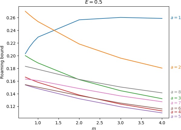
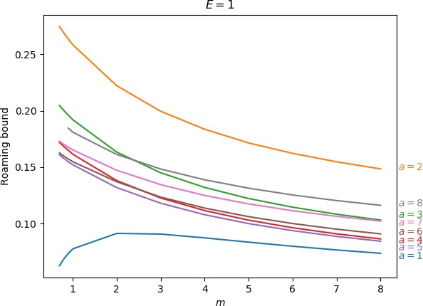
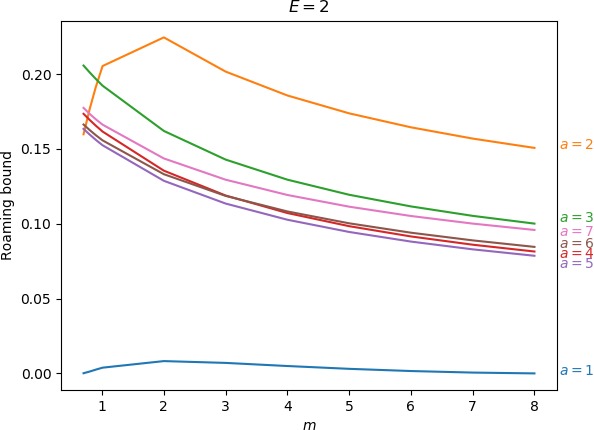
Below we give the upper bound on roaming, which is the ratio of the minimum of the areas γu+i∖γs−o and γs−o∖γu+i to the energy surface volume for r=∞. As explained above, the area γu+i∖γs−o contains all isomerisation and roaming trajectories, while γs−o∖γu+i contains all roaming and nonreactive trajectories. The energy surface volume at r=∞ corresponds to all trajectories in the system with the exception of stable islands, which are not relevant in the context of roaming. This measure does not account for isomerisation trajectories, because these are cut off when they re-enter one of the wells. Since all trajectories with the exception of stable islands must eventually leave the wells and the interaction region, we effectively avoid double-counting. Values of the upper bound can be found in Table tab:2 as well as in Figure fig:9.

We do not provide values for E=0.5 and m>4 due to the large radius of Γo; for E=1, a=8 and m<0.9 due to a bifurcation of Γi around m=0.856 after which DSi no longer delimits the corresponding potential well in a reasonable manner and similarly for E=2 and a=8.

As the values in Table tab:2 show, the prominence of roaming does not evolve in a simple manner. In agreement with conclusions in Sections sec:5, sec:6, sec:7, the proportion of roaming decreases or even disappears for very large and very small masses of the free atom and we known it also recedes in favour of isomerisation with increasing a. Unlike the area of γu+i∖γs−o, which grows monotonically both in m and a, our upper bound on roaming being the smaller of γu+i∖γs−o and γs−o∖γu+i does not. Figure fig:9 suggest that while there is an optimum at a reasonable mass for a=1 and occasionally a=2, the bound otherwise decreases with m with an optimum at a value of m smaller than considered in this work.

The strange evolution of the bound with respect to a, which is shown in Figure fig:9, is probably due to the inaccuracy of the bound. Overall it seems that the proportion of roaming mostly decreases, which is due to prevalence of isomerisation as a increases.

An estimate of the amount of roaming in the system can be obtained via an approximation of the proportion of nonreactive trajectories in γs−o∖γu+i either via a computationally expensive brute force method or from the intersection of invariant manifolds with a surface θ=const that does not suffer from transition between spherical and toric local geometries. Such an estimate is outside of the scope of this work.

E=0.5

\	0.7	0.8	0.9	mH	2	3	4	5	6	7	8	m
1	0.203	0.214	0.222	0.229	0.257	0.260	0.259
2	0.270	0.264	0.259	0.254	0.218	0.196	0.180
3	0.200	0.196	0.192	0.189	0.162	0.145	0.132
4	0.166	0.163	0.161	0.158	0.138	0.124	0.113
5	0.154	0.152	0.150	0.148	0.132	0.119	0.110
6	0.154	0.153	0.152	0.150	0.137	0.125	0.116
7	0.163	0.162	0.162	0.161	0.148	0.137	0.127
8	0.183	0.182	0.180	0.178	0.163	0.151	0.141
a	-	-	-	-	-	-	-

E=1

\	0.7	0.8	0.9	mH	2	3	4	5	6	7	8	m
1	0.063	0.069	0.074	0.078	0.091	0.091	0.087	0.084	0.080	0.077	0.074
2	0.274	0.269	0.264	0.258	0.222	0.200	0.184	0.171	0.162	0.155	0.148
3	0.205	0.200	0.196	0.192	0.163	0.145	0.132	0.122	0.115	0.108	0.103
4	0.172	0.168	0.165	0.161	0.138	0.123	0.112	0.103	0.096	0.091	0.086
5	0.161	0.158	0.155	0.152	0.132	0.118	0.108	0.100	0.094	0.089	0.084
6	0.163	0.160	0.157	0.155	0.137	0.124	0.114	0.106	0.100	0.095	0.091
7	0.173	0.170	0.168	0.165	0.147	0.135	0.125	0.117	0.111	0.106	0.102
8	-	-	0.185	0.181	0.161	0.148	0.139	0.131	0.125	0.120	0.116
a	-	-	-	-	-	-	-	-

E=2

\	0.7	0.8	0.9	mH	2	3	4	5	6	7	8	m
1	0.000	0.001	0.003	0.004	0.008	0.007	0.005	0.003	0.002	0.001	0.000
2	0.160	0.177	0.192	0.205	0.224	0.202	0.186	0.174	0.164	0.157	0.151
3	0.206	0.201	0.197	0.192	0.162	0.143	0.129	0.119	0.112	0.105	0.100
4	0.173	0.169	0.165	0.162	0.135	0.119	0.107	0.098	0.092	0.086	0.081
5	0.163	0.160	0.156	0.152	0.129	0.113	0.103	0.095	0.088	0.083	0.079
6	0.166	0.163	0.159	0.156	0.133	0.119	0.108	0.100	0.094	0.089	0.085
7	0.177	0.173	0.170	0.166	0.144	0.129	0.119	0.111	0.105	0.100	0.096
a	-	-	-	-	-	-	-	-

---

---

From a quantitative perspective we established an upper bound on the prominence of roaming in Chesnavich's CH+4 model. The bound only highlights the intricacy of roaming as a type of dynamics on the verge between isomerisation and nonreactivity. It relies on a generous access to the potential wells to allow reactions as well as a prominent area of high potential that aids sufficient transfer of energy from angular motion to radial motion to prevent isomerisation.

We conclude that it is not possible to choose realistic values of m and a, such that roaming becomes the dominant form of dissociation such as found in acetaldehyde [1]. Therefore the dominance of roaming must be due to other properties of the system than only mass of the free atom and strength of potential coupling of the degrees of freedom. Our investigation shows that roaming is prone to being dominated by other types of dynamics. Therefore the path to dominance of roaming lies in, as our investigation shows, potential wells that are easily accessible by being 'open' in the angular direction to discourage nonreactivity, yet are separated by a sufficiently high isomerisation barrier.

References

1. B. R. Heazlewood et al., “Roaming is the dominant mechanism for molecular products in acetaldehyde photodissociation,” Proc. Nat. Acad. Sci., vol. 105, pp. 12719–12724, 2008.
2. W. J. Chesnavich, “Multiple transition states in unimolecular reactions,” J. Chem. Phys., vol. 84, no. 5, pp. 2615–2619, 1986.
3. D. Townsend et al., “The Roaming Atom: Straying from the Reaction Path in Formaldehyde Decomposition,” Science, vol. 306, no. 5699, pp. 1158–1161, 2004.
4. R. D. van Zee, M. F. Foltz, and C. B. Moore, “Evidence for a second molecular channel in the fragmentation of formaldehyde,” J. Chem. Phys., vol. 99, no. 3, pp. 1664–1673, 1993.
5. J. M. Bowman and B. C. Shepler, “Roaming Radicals,” Annu. Rev. Phys. Chem., vol. 62, pp. 531–553, 2011.
6. P. L. Huston, R. Conte, and J. M. Bowman, “Roaming Under the Microscope: Trajectory Study of Formaldehyde Dissociation,” J. Phys. Chem. A, vol. 120, pp. 5103–5114, 2016.
7. S. Wiggins, L. Wiesenfeld, C. Jaffé, and T. Uzer, “Impenetrable Barriers in Phase-Space,” Phys. Rev. Lett., vol. 86, no. 24, pp. 5478–5481, 2001.
8. T. Uzer, C. Jaffé, J. Palacián, P. Yanguas, and S. Wiggins, “The geometry of reaction dynamics,” Nonlinearity, vol. 15, pp. 957–992, 2002.
9. H. Waalkens and S. Wiggins, “Direct construction of a dividing surface of minimal flux for multi-degree-of-freedom systems that cannot be recrossed,” J. Phys. A, vol. 37, p. L435, 2004.
10. F. A. L. Mauguière et al., “Phase Space Structures Explain Hydrogen Atom Roaming in Formaldehyde Decomposition,” J. Phys. Chem. Lett., vol. 6, no. 20, pp. 4123–4128, 2015.
11. R. S. MacKay and D. C. Strub, “Bifurcations of transition states: Morse bifurcations,” Nonlinearity, vol. 27, no. 5, pp. 859–895, 2014.
12. R. S. MacKay and D. C. Strub, “Morse bifurcations of transition states in bimolecular reactions,” Nonlinearity, vol. 28, no. 12, p. 4303, 2015.
13. F. A. L. Mauguière et al., “Phase space barriers and dividing surfaces in the absence of critical points of the potential energy: Application to roaming in ozone,” J. Chem. Phys., vol. 144, no. 5, p. 54107, 2016.
14. M. J. T. Jordan, S. C. Smith, and R. G. Gilbert, “Variational transition state theory: A simple model for dissociation and recombination reactions of small species,” J. Phys. Chem. , vol. 95, no. 22, pp. 8685–8694, 1991.
15. F. A. L. Mauguière, P. Collins, G. S. Ezra, S. C. Farantos, and S. Wiggins, “Roaming dynamics in ion-molecule reactions: Phase space reaction pathways and geometrical interpretation,” J. Chem. Phys., vol. 140, no. 13, p. 134112, 2014.
16. F. A. L. Mauguière, P. Collins, G. S. Ezra, S. C. Farantos, and S. Wiggins, “Multiple transition states and roaming in ion–molecule reactions: A phase space perspective,” Chem. Phys. Lett., vol. 592, pp. 282–287, 2014.