
Three degree-of-freedom Barbanis system
Introduction
It is well-known now that the paradigm of escape from a potential well and the topology of phase space structures that mediate such escape are used in a broad array of problems such as isomerization of molecular clusters [1], reaction rates in chemical physics [2], [3], ionization of a hydrogen atom under electromagnetic field in atomic physics [4], transport of defects in solid state and semiconductor physics [5], buckling modes in structural mechanics [6], [7], ship motion and capsize [8], [9], [10], escape and recapture of comets and asteroids in celestial mechanics [11], [12], [13], and escape into inflation or re-collapse to singularity in cosmology [14]. As such a method that can identify the high dimensional phase space structures using low dimensional surface as probes can aid in quantifying the escape rates. These low dimensional surfaces has been shown to be of as reactive islands in chemical physics and lead to insights into sampling rare transition events [15], [16]. However, to benchmark the methodology, we first applied it to linear systems where the closed-form analytical expression of the phase space structures is known [17]. As the next step, in this article, we will focus on nonlinear Hamiltonian systems which have been extensively studied as "built by hand" models of galactic dynamics and for demonstrating quantum dynamical tunneling [18], [19], [20], [21], [22], [23], [24], [25], [26], [27]. The nonlinear Hamiltonian systems considered here have an underlying Hénon-Heiles type potential with the simplest form of nonlinearity, and show regular, quasi-periodic, and chaotic trajectories along with bifurcations of periodic orbits. A Hénon-Heiles type potential has a well with bottlenecks connecting the region of bounded motion (trapped region) to unbounded motion (escape off to infinity), and have rotational symmetry. In addition, these Hénon-Heiles type potentials are studied as first benchmark nonlinear systems in applying new phase space transport methods to astrophysical and molecular motion. In this article, we will present verification of a method that uses trajectory diagnostic on a low dimensional surface for revealing the phase space structures in 4 or more dimensions.
Conservative dynamics on an open potential well has received considerable attention because the phase space structures, normally hyperbolic invariant manifolds (NHIM) and its invariant manifolds, explain the intricate fractal structure of ionization rates [28], [29], [30]. Furthermore, the discrepancies in observed and predicted ionization rates in atomic systems has also been explained by accounting for the topology of the phase space structures. These have been connected with the breakdown of ergodic assumption that is the basis for using ionization and dissociation rate formulae [31]. This rich literature on chaotic escape of electrons from atoms sets a precedent for applying new methods for finding NHIM and its invariant manifolds in Hamiltonian with open potential wells (missing reference).
As we noted earlier, trajectory diagnostic methods which can probe phase space to detect the high dimensional invariant manifolds have potential to be of use in many degrees-of-freedom models. One such method is the Lagrangian descriptors (LDs) that can reveal phase space structures by encoding geometric property of trajectories (such as, phase space arc length, configuration space distance or displacement, cumulative action or kinetic energy) initialised on a two dimensional surface [32], [33], [34], [35]. The method was originally developed in the context of Lagrangian transport in time-dependent two dimensional fluid mechanics. However, it has also been successful in locating transition state trajectory in chemical reactions [36], [37], [38]. Besides, also being applicable to both Hamiltonian and non-Hamiltonian systems, as well as to systems with arbitrary time-dependence such as stochastic and dissipative forces, and geophysical data from satellite and numerical simulations [39], [40], [41], [35], [42].
We present the capability of Lagrangian descriptors for revealing the high dimensional phase space structures that are of interest in nonlinear Hamiltonian systems with index-1 saddle. These phase space structures include normally hyperbolic invariant manifolds (NHIM) and their stable and unstable manifolds, and act as codimenision-1 barriers to phase space transport. The method is applied to classical two and three degrees-of-freedom Hamiltonian systems which have implications for myriad applications in physics and chemistry.
The method of Lagrangian descriptor (LD) is straightforward to implement computationally and it provides a "high resolution" method for exploring the influence of high dimensional phase space structure on trajectory behaviour. The method of LD takes an opposite approach to that of classical Lyapunov exponent type calculations by emphasizing the initial conditions of trajectories, rather than their advected locations that is involved in calculating normalized rate of divergence. This is achieved by considering a two dimensional section of the full phase space and discretizing with a dense grid of initial conditions. Even though the trajectories wander off in the phase space, as the initial conditions evolve in time, there is no loss in resolution of the two dimensional section. In contrast to inferring the phase space structures from Poincaré sections, LD plots do not suffer from loss of resolution since the affects of the structure are encoded in the initial conditions and there is no need for the trajectory to return to the section. Our objective is to clarify the use of Lagrangian descriptors as a diagnostic on two dimensional sections of high dimensional phase space structures. This diagnostic is also meant to be used as the preliminary step in computing the NHIM, their stable and unstable manifolds using other computational means [43], [44], [45]. In this article, we will present the method's capability to detect the high dimensional phase space structures such as the NHIM, their stable, and unstable manifolds in 2 and 3 DoF Hamiltonian systems.
Development of the Problem [[sec:model_prob_2dof]]{#sec:model_prob_2dof label="sec:model_prob_2dof"}
The model system to consider is the coupled harmonic potential in 3 dimensions and underlying a 3 degrees-of-freedom system in [46], [47]. The Hamiltonian is given by
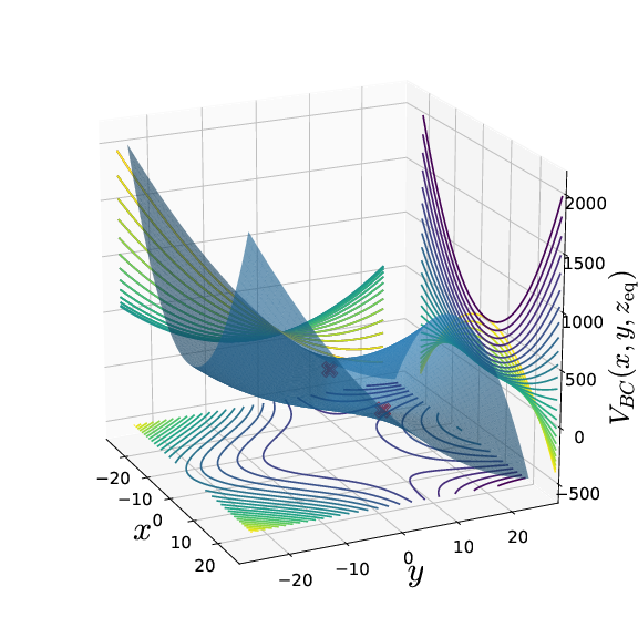
\begin{align} \mathcal{H}(x,y,z,p_x,p_y,p_z) = T(p_x, p_y, p_z) + V_{\rm BC}(x,y,z) = \frac{1}{2}p_x^2 + \frac{1}{2}p_y^2 + \frac{1}{2}p_z^2 + \frac{1}{2}\omega_x^2 x^2 + \frac{1}{2}\omega_y^2 y^2 + \frac{1}{2}\omega_z^2 z^2 - \epsilon x^2y - \eta x^2 z \label{eqn:Hamiltonian_BC_3dof} \end{align}where $\omega_x^2, \omega_y^2, \omega_z^2, \epsilon, \eta$ are the parameters related to the coupled harmonic 3 dimensional potential energy function [47]. In this study, we will fix the parameters to be $\omega_x^2 = 0.9, \omega_y^2 = 1.6, \omega_z^2 = 0.4, \epsilon = 0.08, \eta = 0.01$. The two index-1 saddle equilibria (as shown in the App. 6{reference-type="ref" reference="sect:coupled_3dof"}) of the Hamiltonian vector field [eqn:three_dof_Barbanis]{reference-type="eqref" reference="eqn:three_dof_Barbanis"} are located at
\begin{equation} \left(\pm \frac{\omega_x\omega_y\omega_z}{\sqrt{2(\epsilon^2\omega_z^2 + \eta^2\omega_y^2)}}, \frac{\epsilon \omega_x^2\omega_z^2}{2(\epsilon^2\omega_z^2 + \eta^2\omega_y^2)}, \frac{\eta \omega_x^2\omega_y^2}{2(\epsilon^2\omega_z^2 + \eta^2\omega_y^2)}, 0, 0, 0 \right) \label{eqn:eq_pt_BC_3dof} \end{equation}and the total energy is $$E_c = \frac{1}{8} \omega_x^2 \frac{\omega_x^2 \omega_y^2 \omega_z^2}{ \left( \epsilon^2 \omega_z^2 + \eta^2 \omega_y^2 \right)}.$$ The equilibrium point at $(0,0,0,0,0,0)$ is stable and has total energy $0$. For the parameters used in this study, the equilibrium points are located at $\left( \pm 10.290, 5.294, 2.647, 0, 0, 0 \right)$ and $\left( 0, 0, 0, 0, 0, 0 \right)$ and have total energy, $E_c \approx 23.824$ and $E = 0$, respectively.
We show the isopotential contours of the potential energy function at fixed value of $z_{\rm eq}$ in Fig. [fig:Barbanis_Contopoulos_3dof]{reference-type="ref" reference="fig:Barbanis_Contopoulos_3dof"} along with the Hill's regions for positive excess energy, $\Delta E = 6.000$ and projected on the configuration space coordinates at the equilibrium point.
 {width="25.00000%"}\
 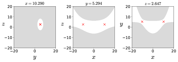 {width="70.00000%"}
[[fig:Barbanis_Contopoulos_3dof]]{#fig:Barbanis_Contopoulos_3dof
label="fig:Barbanis_Contopoulos_3dof"}
{width="70.00000%"}
[[fig:Barbanis_Contopoulos_3dof]]{#fig:Barbanis_Contopoulos_3dof
label="fig:Barbanis_Contopoulos_3dof"}
Fig. 2. (a) Potential energy function underlying the coupled harmonic Hamiltonian~\eqref{eqn:Hamiltonian_BC3dof} at $z{\rm eq} = 2.647$ as isopotential contour and surface. (b) Hill's region for excess energy, $\Delta E = 6.000$ and projected on the configuration space coordinates at the equilibrium point. We note here that the potential energy surface and the Hill's region is plotted by fixing one of the configuration coordinates at the equilibrium point.
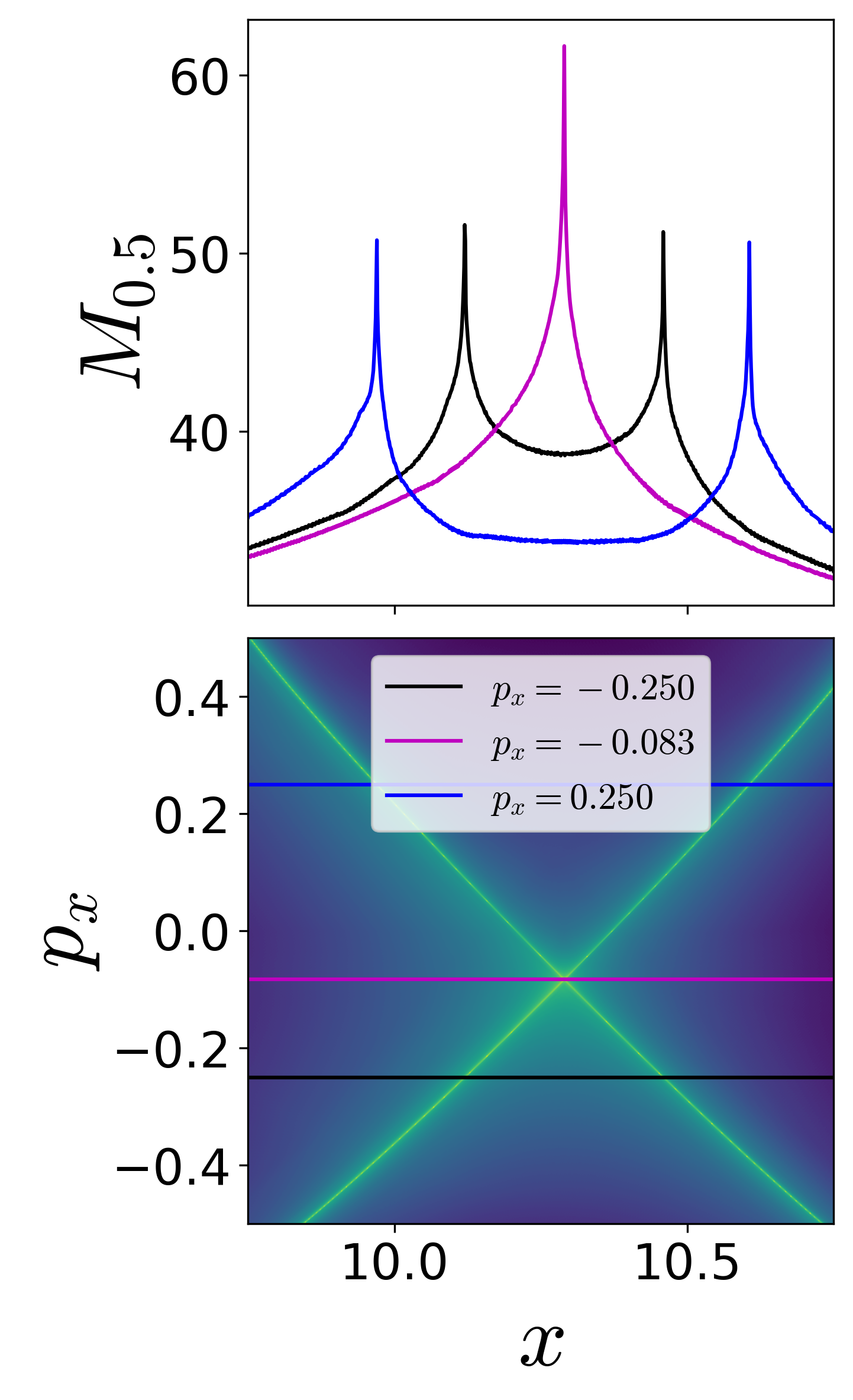
Since this model system is conservative 3 DoF Hamiltonian, that is the phase space is $\mathbb{R}^6$, the energy surface is five dimensional, the dividing surface is four dimensional, and the normally hyperbolic invariant manifold (NHIM) is three dimensional, or precisely 3-sphere, and its invariant manifolds are four dimensional, or precisely $\mathbb{R}^1 \times \mathbb{S}^3$ or spherical cylinders [48]. Now, if we consider the intersection of a two-dimensional section with the five dimensional energy surface in $\mathbb{R}^6$, we would obtain the one-dimensional energy boundary on the surface. We will focus our study near the bottleneck by considering the isoenergetic two dimensional surfaces
\begin{align} U_{xp_x}^+ = & \left\{ (x, y, z, p_x, p_y, p_z) \; | \; y = y_{\rm eq}, z = z_{\rm eq}, \; p_y = 0, \; p_z(x, y, z, p_x, p_y; e) > 0 \right\} \label{eqn:Barbanis3dof_uxpx}\\ U_{yp_y}^+ = & \left\{ (x, y, z, p_x, p_y, p_z) \; | \; x = x_{\rm eq}, z = z_{\rm eq}, \; p_x = 0, \; p_z(x, y, z, p_x, p_y; e) > 0 \right\} \label{eqn:Barbanis3dof_uypy}\\ U_{zp_z}^+ = & \left\{ (x, y, z, p_x, p_y, p_z) \; | \; x = x_{\rm eq}, y = y_{\rm eq}, \; p_x = 0, \; p_y(x, y, z, p_x, p_z; e) > 0 \right\} \label{eqn:Barbanis3dof_uzpz} % \label{eqn:Barbanis3dof_sos_near_saddle} \end{align}In this 3 DoF system, detecting points on the three dimensional NHIM and four dimensional invariant manifolds will constitute finding their intersection with the above two dimensional surfaces.
Revealing Phase Space Structures
The Lagrangian descriptor based approach for detecting NHIM in 2 DoF system can now be applied to the 3 DoF system [eqn:Hamiltonian_BC_3dof]{reference-type="eqref" reference="eqn:Hamiltonian_BC_3dof"}. On the five dimensional energy surface, the phase space structures such as the NHIM and its invariant manifolds are three and four dimensional, respectively [48]. As noted earlier, direct visualization techniques will fall short in 4 or more DoF systems even if they are successful in 2 and 3 DoF. So, LD based approach can be used to detect points on a NHIM and its invariant manifolds using low dimensional probe which are based on trajectory diagnostic on an isoenergetic two dimensional surface.
It is to be noted that the increase in phase space dimension, leads to a polynomial scaling in the number of coordinate pairs (that is $2N(2N-1)(N-1)$ coordinate pairs for $N$ DoF system) and is thus, impractical to present the procedure on all the combination of coordinates. We will present the results for the three configuration space coordinates by combining each with its corresponding momentum coordinate.
On these isoenergetic surfaces, we compute the variable integration time Lagrangian descriptor for small excess energy, $\Delta E \approx 0.176$, or total energy $E = 24.000$, and show the contour maps in Fig. [fig:Barbanis3dof_M_pxpypz]{reference-type="ref" reference="fig:Barbanis3dof_M_pxpypz"}. The maxima identifying the points on the NHIM and its invariant manifolds can be visualized using one dimensional slices for constant momenta. This indicates clearly the initial conditions in the phase space (points on the isoenergetic two dimensional surfaces in $\mathbb{R}^6$, for example [eqn:Barbanis3dof_uxpx]{reference-type="eqref" reference="eqn:Barbanis3dof_uxpx"}) that do not leave the saddle region.
 {width="33.00000%"}\
 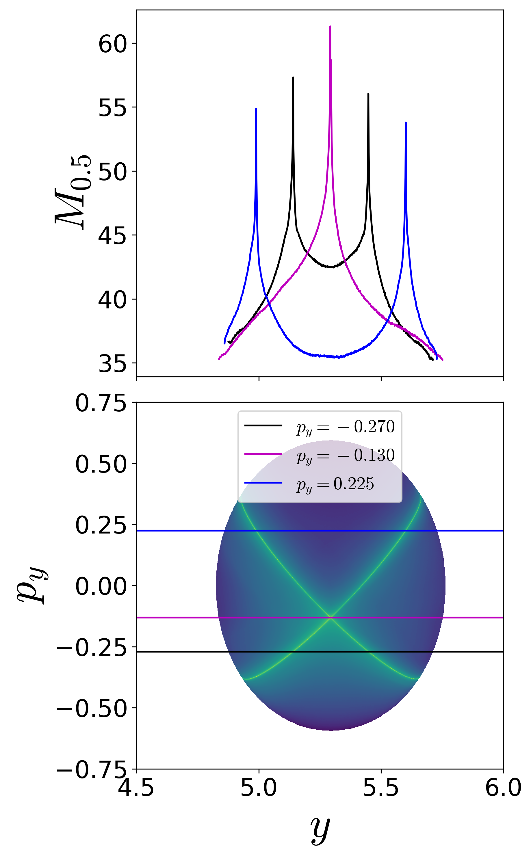 {width="33.00000%"}\
 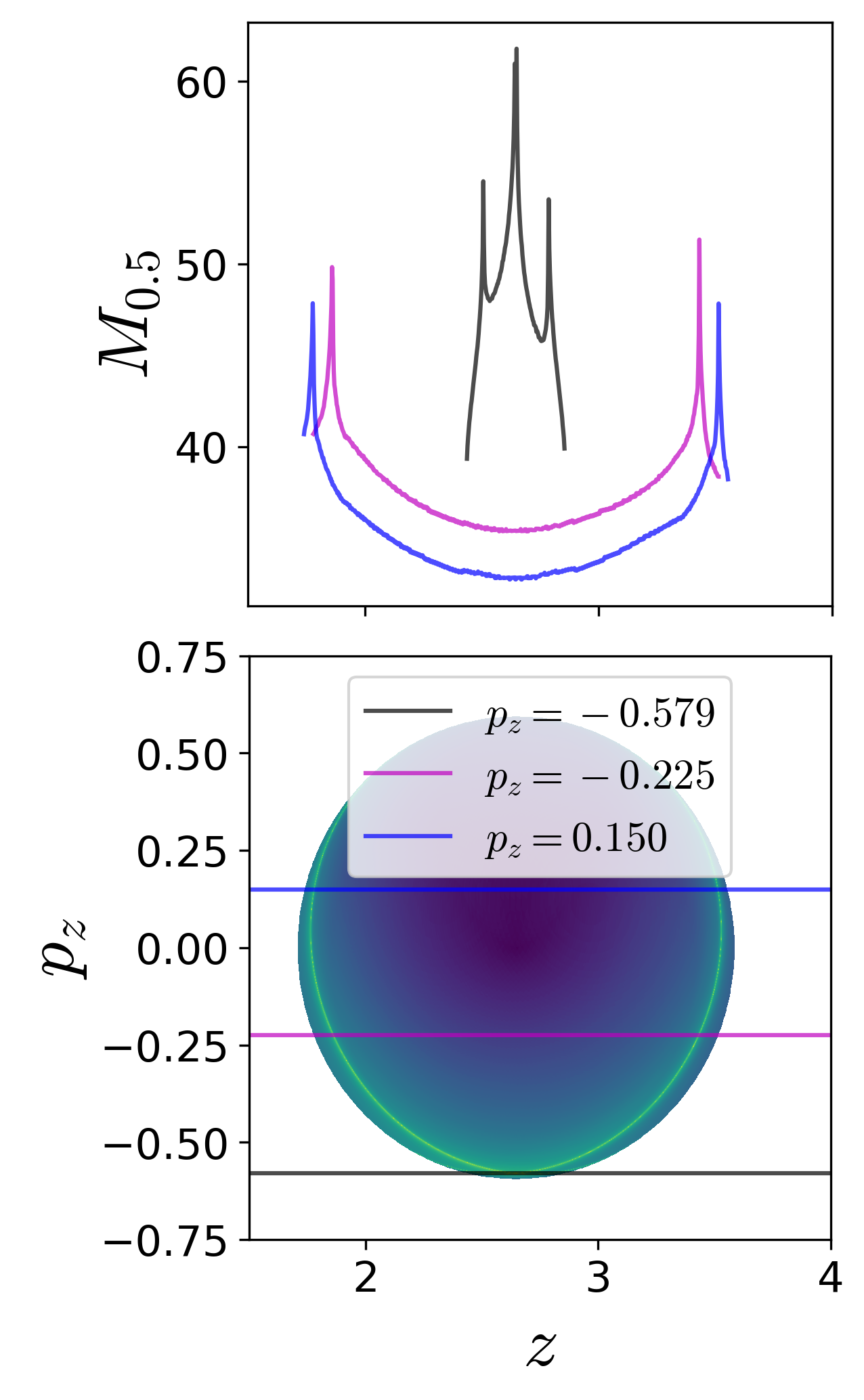 {width="33.00000%"}
Fig. 5. Detecting points on the NHIM using variable integration time Lagrangian descriptor on the two dimensional surfaces (a) $U_{xp_x}^+$~\eqref{eqn:Barbanis3dofuxpx}, (b) $U{yp_y}^+$~\eqref{eqn:Barbanis3dof_uypy}, and (c) $U_{zp_z}^+$~\eqref{eqn:Barbanis3dof_uzpz} at excess energy $\Delta E \approx 0.176$ or total energy $E = 24.000$. For this energy value, the saddle region, as defined in Eqn.~\eqref{eqn:var_time_qs}, is taken to be $q_s = [9,12] \times [2.5,7.5] \times [1,4]$ and $\tau = 50$.
{width="33.00000%"}
Fig. 5. Detecting points on the NHIM using variable integration time Lagrangian descriptor on the two dimensional surfaces (a) $U_{xp_x}^+$~\eqref{eqn:Barbanis3dofuxpx}, (b) $U{yp_y}^+$~\eqref{eqn:Barbanis3dof_uypy}, and (c) $U_{zp_z}^+$~\eqref{eqn:Barbanis3dof_uzpz} at excess energy $\Delta E \approx 0.176$ or total energy $E = 24.000$. For this energy value, the saddle region, as defined in Eqn.~\eqref{eqn:var_time_qs}, is taken to be $q_s = [9,12] \times [2.5,7.5] \times [1,4]$ and $\tau = 50$.
Implications for reaction dynamics
References
- T. Komatsuzaki and R. S. Berry, “Dynamical hierarchy in transition states: Why and how does a system climb over the mountain?,” P. Natl. Acad. Sci. USA, vol. 98, no. 14, pp. 7666–7671, 2001.
- T. Komatsuzaki and R. S. Berry, “Regularity in chaotic reaction paths. I. Ar6,” The Journal of Chemical Physics, vol. 110, no. 18, pp. 9160–9173, 1999.
- S. Wiggins, L. Wiesenfeld, C. Jaffé, and T. Uzer, “Impenetrable Barriers in Phase Space,” Phys. Rev. Lett., vol. 86, pp. 5478–5481, 2001.
- C. Jaffé, D. Farrelly, and T. Uzer, “Transition state theory without time-reversal symmetry: chaotic ionization of the hydrogen atom,” Phys. Rev. Lett., vol. 84, pp. 610–613, 2000.
- B. Eckhardt, “Transition state theory for ballistic electrons,” J. Phys. A-Math. Gen., vol. 28, no. 12, p. 3469, 1995.
- P. Collins, G. S. Ezra, and S. Wiggins, “Isomerization dynamics of a buckled nanobeam,” Phys. Rev. E, vol. 86, no. 5, p. 056218, Nov. 2012.
- J. Zhong, L. N. Virgin, and S. D. Ross, “A tube dynamics perspective governing stability transitions: An example based on snap-through buckling,” Int. J. Mech. Sci., vol. 000, no. May, pp. 1–16, 2018.
- L. N. Virgin, “Approximate criterion for capsize based on deterministic dynamics,” Dynamics and Stability of Systems, vol. 4, no. 1, pp. 56–70, 1989.
- J. M. T. Thompson and J. R. de Souza, “Suppression of escape by resonant modal interactions: in shell vibration and heave-roll capsize,” Proc. R. Soc. Lond. A, vol. 452, pp. 2527–2550, 1996.
- S. Naik and S. D. Ross, “Geometry of escaping dynamics in nonlinear ship motion,” Commun. Nonlinear Sci., vol. 47, pp. 48–70, 2017.
- C. Jaffé, S. D. Ross, M. W. Lo, J. E. Marsden, D. Farrelly, and T. Uzer, “Statistical theory of asteroid escape rates,” Physical Review Letters, vol. 89, no. 1, p. 011101, 2002.
- M. Dellnitz et al., “Transport of Mars-crossing asteroids from the quasi-Hilda region,” Physical Review Letters, vol. 94, p. 231102, 2005.
- S. D. Ross, “Statistical theory of interior-exterior transition and collision probabilities for minor bodies in the solar system,” in Libration Point Orbits and Applications, G. Gómez, M. W. Lo, and J. J. Masdemont, Eds. World Scientific, 2003, pp. 637–652.
- H. P. de Oliveira, A. M. Ozorio de Almeida, I. Damião Soares, and E. V. Tonini, “Homoclinic chaos in the dynamics of a general Bianchi type-IX model,” Phys. Rev. D, vol. 65, no. 8, p. 9, 2002.
- S. Patra and S. Keshavamurthy, “Classical-quantum correspondence in a model for conformational dynamics: Connecting phase space reactive islands with rare events sampling,” Chemical Physics Letters, vol. 634, pp. 1–10, Aug. 2015.
- S. Patra and S. Keshavamurthy, “Detecting reactive islands using Lagrangian descriptors and the relevance to transition path sampling,” Physical Chemistry Chemical Physics, vol. 20, no. 7, pp. 4970–4981, 2018.
- S. Naik, Garcı́a-Garrido Vı́ctor J, and S. Wiggins, “Finding NHIM: Identifying High Dimensional Phase Space Structures in Reaction Dynamics using Lagrangian Descriptors,” arXiv preprint arXiv:1903.10264, 2019.
- B. Barbanis, “On the isolating character of the ‘third’ integral in a resonance case,” The Astronomical Journal, vol. 71, p. 415, Aug. 1966.
- P. Brumer and J. W. Duff, “A variational equations approach to the onset of statistical intramolecular energy transfer,” The Journal of Chemical Physics, vol. 65, no. 9, pp. 3566–3574, Nov. 1976.
- M. J. Davis and E. J. Heller, “Semiclassical Gaussian basis set method for molecular vibrational wave functions,” The Journal of Chemical Physics, vol. 71, no. 8, pp. 3383–3395, Oct. 1979.
- E. J. Heller, E. B. Stechel, and M. J. Davis, “Molecular spectra, Fermi resonances, and classical motion,” The Journal of Chemical Physics, vol. 73, no. 10, pp. 4720–4735, Nov. 1980.
- B. A. Waite and W. H. Miller, “Mode specificity in unimolecular reaction dynamics: The Hénon-Heiles potential energy surface,” The Journal of Chemical Physics, vol. 74, no. 7, pp. 3910–3915, Apr. 1981.
- R. Kosloff and S. A. Rice, “Dynamical correlations and chaos in classical Hamiltonian systems,” The Journal of Chemical Physics, vol. 74, no. 3, pp. 1947–1955, Feb. 1981.
- G. Contopoulos and P. Magnenat, “Simple three-dimensional periodic orbits in a galactic-type potential,” Celestial Mechanics, vol. 37, no. 4, pp. 387–414, Dec. 1985.
- M. Founargiotakis, S. C. Farantos, G. Contopoulos, and C. Polymilis, “Periodic orbits, bifurcations, and quantum mechanical eigenfunctions and spectra,” The Journal of Chemical Physics, vol. 91, no. 3, pp. 1389–1402, Aug. 1989.
- B. Barbanis, “Escape regions of a quartic potential,” Celestial Mechanics and Dynamical Astronomy, vol. 48, no. 1, pp. 57–77, 1990.
- D. Babyuk, R. E. Wyatt, and J. H. Frederick, “Hydrodynamic analysis of dynamical tunneling,” The Journal of Chemical Physics, vol. 119, no. 13, pp. 6482–6488, Oct. 2003.
- K. A. Mitchell, J. P. Handley, B. Tighe, J. B. Delos, and S. K. Knudson, “Geometry and topology of escape. I. Epistrophes,” Chaos: An Interdisciplinary Journal of Nonlinear Science, vol. 13, no. 3, pp. 880–891, Sep. 2003.
- K. A. Mitchell, J. P. Handley, J. B. Delos, and S. K. Knudson, “Geometry and topology of escape. II. Homotopic lobe dynamics,” Chaos: An Interdisciplinary Journal of Nonlinear Science, vol. 13, no. 3, pp. 892–902, Sep. 2003.
- K. A. Mitchell, J. P. Handley, B. Tighe, A. Flower, and J. B. Delos, “Chaos-Induced Pulse Trains in the Ionization of Hydrogen,” Physical Review Letters, vol. 92, no. 7, Feb. 2004.
- N. De Leon and B. J. Berne, “Intramolecular rate process: Isomerization dynamics and the transition to chaos,” The Journal of Chemical Physics, vol. 75, no. 7, pp. 3495–3510, Oct. 1981.
- J. A. J. Madrid and A. M. Mancho, “Distinguished trajectories in time dependent vector fields,” Chaos, vol. 19, p. 013111, 2009.
- C. Mendoza and A. M. Mancho, “The hidden geometry of ocean flows,” Phys. Rev. Lett., vol. 105, no. 3, p. 038501, 2010.
- A. M. Mancho, S. Wiggins, J. Curbelo, and C. Mendoza, “Lagrangian Descriptors: A Method for Revealing Phase Space Structures of General Time Dependent Dynamical Systems.,” Communications in Nonlinear Science and Numerical, vol. 18, pp. 3530–3557, 2013.
- C. Lopesino, F. Balibrea-Iniesta, V. J. García-Garrido, S. Wiggins, and A. M. Mancho, “A Theoretical Framework for Lagrangian Descriptors,” International Journal of Bifurcation and Chaos, vol. 27, no. 01, p. 1730001, 2017.
- F. Balibrea-Iniesta, C. Lopesino, S. Wiggins, and A. M. Mancho, “Lagrangian Descriptors for Stochastic Differential Equations: A Tool for Revealing the Phase Portrait of Stochastic Dynamical Systems,” International Journal of Bifurcation and Chaos, vol. 26, no. 13, p. 1630036, 2016.
- G. T. Craven, A. Junginger, and R. Hernandez, “Lagrangian descriptors of driven chemical reaction manifolds,” Physical Review E, vol. 96, no. 2, p. 022222, 2017.
- A. Junginger and R. Hernandez, “Lagrangian descriptors in dissipative systems,” Physical Chemistry Chemical Physics, vol. 18, no. 44, pp. 30282–30287, 2016.
- A. de la Cámara, A. M. Mancho, K. Ide, E. Serrano, and C. R. Mechoso, “Routes of transport across the Antarctic polar vortex in the southern spring,” J. Atmos. Sci., vol. 69, no. 2, pp. 753–767, 2012.
- C. Mendoza, A. M. Mancho, and S. Wiggins, “Lagrangian descriptors and the assessment of the predictive capacity of oceanic data sets,” Nonlinear Processes in Geophysics, vol. 21, no. 3, pp. 677–689, 2014.
- Garcı́a-Garrido V. J., A. M. Mancho, and S. Wiggins, “A dynamical systems approach to the surface search for debris associated with the disappearance of flight MH370.,” Nonlin. Proc. Geophys., vol. 22, pp. 701–712, 2015.
- A. G. Ramos et al., “Lagrangian coherent structure assisted path planning for transoceanic autonomous underwater vehicle missions.,” Scientfic Reports, vol. 4, p. 4575, 2018.
- A. Junginger et al., “Transition state geometry of driven chemical reactions on time-dependent double-well potentials,” Physical Chemistry Chemical Physics, vol. 18, no. 44, pp. 30270–30281, 2016.
- R. Bardakcioglu, A. Junginger, M. Feldmaier, J. Main, and R. Hernandez, “Binary contraction method for the construction of time-dependent dividing surfaces in driven chemical reactions,” Physical Review E, vol. 98, no. 3, Sep. 2018.
- G. S. Ezra and S. Wiggins, “Sampling Phase Space Dividing Surfaces Constructed from Normally Hyperbolic Invariant Manifolds (NHIMs),” The Journal of Physical Chemistry A, vol. 122, no. 42, pp. 8354–8362, 2018.
- G. Contopoulos, S. C. Farantos, H. Papadaki, and C. Polymilis, “Complex unstable periodic orbits and their manifestation in classical and quantum dynamics,” Physical Review E, vol. 50, no. 6, pp. 4399–4403, Dec. 1994.
- S. C. Farantos, “POMULT: A program for computing periodic orbits in hamiltonian systems based on multiple shooting algorithms,” Computer Physics Communications, vol. 108, no. 2-3, pp. 240–258, Feb. 1998.
- S. Wiggins, “The role of normally hyperbolic invariant manifolds (NHIMS) in the context of the phase space setting for chemical reaction dynamics,” Regular and Chaotic Dynamics, vol. 21, no. 6, pp. 621–638, Nov. 2016.